More than 23% of agricultural cooperatives are more than 100 years old and 77% are more than 50 years old. Part of the clientele for those cooperatives are young producers. Almost 300,000 farmers (9% of the total) are under 35 years of age. This small but growing segment of the farm population often has limited access to land and credit and has greater financial vulnerability. Old cooperatives and young farmers can clearly benefit from each other but there are challenges involved in successfully matching the two.
Most legacy U.S. agricultural cooperatives operate under the open membership model where members invest in the business by receiving a portion of profits as revolving equity. That structure is young producer friendly in that it allows membership without a large up-front investment. On the other hand, the benefit stream from a cooperative is long-term in nature. Revolving equity patronage only turns into cash after a multi-year delay, and unlike corporate stock, cooperative equity is non-tradable and non-liquid. Agricultural cooperatives may have to re-think long revolving periods if they want to appeal to young producers.
Agricultural cooperatives are also user-controlled, and most cooperatives are eager to have young producers serve on their boards of directors. Unfortunately, young producers may be reluctant to join the board due to the competing use of their time from farm, family and off-farm work obligations. Agricultural cooperatives need new blood and new ideas. They may have to explore new, and less time-demanding, options to involve younger producers.
Despite these challenges, old cooperative and young producers can help each other. Agricultural cooperatives are constantly regenerating themselves and they need new members to create new equity. Young producers face operational and financial challenges. They need secure market access and improved profitability from supply chain ownership. Agricultural cooperatives were formed to allow producers to collectively accomplish what they could not do on their own.
While it is true that young producers may desire a different set of products and services relative to their more experienced brethren, they still represent the future of agricultural cooperatives. For example, young producers may be more interested in input financing and less interested in pre-pay discounts. Their participation may represent new opportunities and new risks for cooperatives. Young producers also tend to be technology savvy. Cooperatives and young producers might make excellent partners in the journey to evaluate and adopt new technologies.
Established cooperatives can benefit from young producers, and young producers can benefit from established cooperatives. Perhaps both sides can explore these opportunities together!
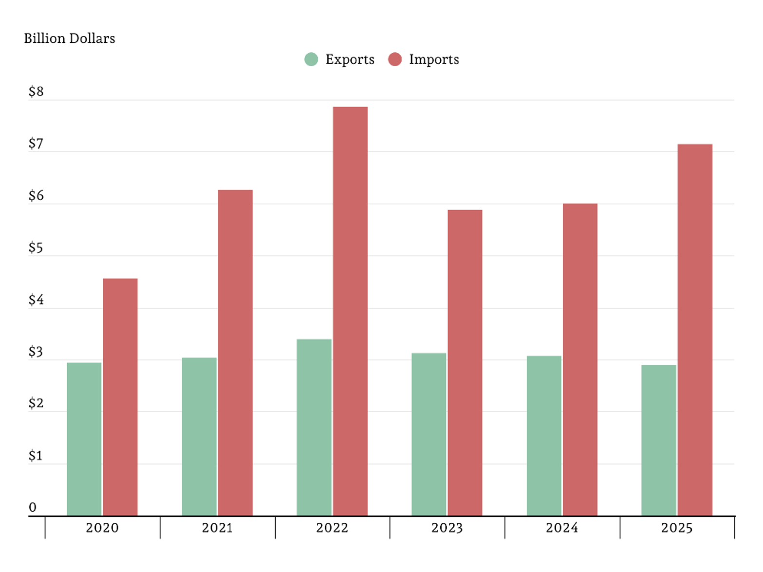
Another trade agreement framework was announced by the White House a few weeks ago, this time with Indonesia. The released statement explains that tariffs on 99 percent of exports from the United States to Indonesia will be removed, as well as addressing non-tariff barriers. In exchange, tariffs will remain at 19 percent for imports from Indonesia. U.S. agricultural imports from Indonesia reached $7.14 billion in 2025, with exports to the country lagging behind at $2.89 billion, which makes Indonesia the 9th largest source of U.S. agricultural imports and 12th largest export destination.
Source: Global Agricultural Trading System (GATS), USDA/FAS
Exports to Indonesia are dominated by oilseeds which makeup over a third of agricultural export value at $1.14 billion. An additional $752 million of exported products were grains and feed. Dairy products accounted for $221 million of the $454 million of animal products exported to Indonesia. Following these main groups are cotton ($146 million), ag chemicals ($58 million), and fish ($55 million).
Graph 2. U.S. Agricultural Exports to Indonesia, 2025
Source: Global Agricultural Trading System (GATS), USDA/FAS
On top of being the most exported agricultural category, oilseed products led imports from Indonesia. Palm oil and palm kernel oil together made up $2.03 billion of the $3.11 billion in oilseed product imports. Fish, primarily shellfish, accounted for a quarter of agricultural imports with $1.86 billion in imports, followed by cocoa and coffee. Overall, Indonesia seems like a very promising market for agricultural products.
Graph 3. U.S. Agricultural Imports from Indonesia, 2025
Source: Global Agricultural Trading System (GATS), USDA/FAS
Sources
Foreign Agricultural Service (FAS). Global Agricultural Trade System (GATS). Online database. Online public database accessed February 2025.
The White House. “Fact Sheet: Trump Administration Finalizes Trade Deal With Indonesia.” February 19, 2025. https://www.whitehouse.gov/fact-sheets/2026/02/fact-sheet-trump-administration-finalizes-trade-deal-with-indonesia/.
Brazil’s 2025/26 soybean crop is headed for a record near 6.6 billion bushels (USDA, 2026). Maples (2026) laid out the fundamentals in Southern Ag Today earlier this season. But as the season has unfolded, the key question for U.S. producers is no longer whether Brazil has soybeans. It is whether Brazil can move them to market as smoothly as the headline crop suggests. Three forces suggest otherwise: logistics frictions are disrupting exports at peak season; geopolitical shocks are raising costs across the supply chain; and a structural rise in domestic crushing is keeping more of the crop inside the country.
The first pressure is timing and logistics. Heavy rains in the Center-West slowed harvest while drought in the South trimmed yields. By mid-March, Brazil’s soybean harvest was running 10.6 percentage points behind the same point last year (Figure 1). About 60% of Brazil’s soybeans move to port by truck, yet only about 14% of the country’s roads are paved (Salin, 2025). A phytosanitary dispute with China compounded the problem: Brazil increased inspections on soybeans bound for China at Beijing’s request, Cargill paused exports to China, and longer certification waits raised both demurrage and freight costs (MAPA, 2026).
The second pressure is cost. Brazil imports more than 80% of its fertilizer (ANDA, 2026), and nearly 30% of global fertilizer exports transit the Strait of Hormuz (FAO, 2026). The closure stranded roughly a million metric tons and sent diesel prices surging in rural Brazil. Because the soybean crop was largely fertilized before the shock, the immediate input-cost pressure falls more on safrinha (second crop) corn and on 2026/27 budgets. But freight costs hit now: bunker fuel prices have surged as the Middle East conflict disrupts supply to Singapore, the world’s largest ship-refueling hub (Bloomberg, 2026).
Beneath these disruptions, a structural shift is changing the soybean balance sheet. Domestic crushing is projected to reach a record 2.26 billion bushels, up about 50% from a decade ago (ABIOVE, 2026). Biodiesel policy is one reason. Brazil’s blending mandate has risen from B7 (or 7%) in 2016 to B15 (or 15%) in 2025, and soybean-oil-based biodiesel production has more than doubled, from about 0.8 billion gallons to 1.9 billion as shown in Figure 2 (ANP/ABIOVE, 2026). More beans crushed at home means fewer whole soybeans available for export.
Two regulatory shifts add nuance. Cargill, ADM, and Bunge withdrew from the Amazon Soy Moratorium in early 2026 after a Mato Grosso state law penalized companies adhering to environmental agreements exceeding federal requirements. Their exit came as the EU Deforestation Regulation (EUDR) is set to enter into force. That collision could create openings for U.S. soy in Europe. Meanwhile, the EU-Mercosur trade agreement would give Brazilian soy preferential European access, but a legal challenge could delay implementation (Council of the European Union, 2026).
Brazil still has an enormous crop. But large production does not guarantee maximum export pressure. Fertilizer costs are higher. Bunker fuel is tight. Port roads are congested. Ships face delays at port. And a growing share of Brazil’s soybeans are staying at home to be crushed domestically. In 2026, the key gap is between Brazil’s ability to grow soybeans and its ability to move them efficiently. That gap is where the competitive opportunity for U.S. producers may emerge.
Figure 1. Brazil Crop Progress Is Running Behind Last Year’s Pace
Note: Soybean harvest and safrinha corn planting as a percentage of total area, week ending March 14. The soybean harvest trailed the prior year by 10.6 percentage points; safrinha corn planting lagged by 4.1 percentage points. Source: CONAB (2026b).
Figure 2. Soybean-Oil-Based Biodiesel Production in Brazil Has More Than Doubled Since 2015
Note: Annual biodiesel production from soybean oil in billion gallons, 2008 through 2025. Production rose from about 0.2 billion gallons in 2008 to 0.8 billion in 2015 and 1.9 billion in 2025. Labels indicate Brazil’s national biodiesel blending mandate, expressed as the share of biodiesel required in commercial diesel fuel: B2 = 2%, B5 = 5%, B7 = 7%, B8 = 8%, B10 = 10%, B14 = 14%, B15 = 15%. Soybean oil accounts for roughly 70–75% of all Brazilian biodiesel feedstock. Source: ANP/ABIOVE (2026).
References
Associação Brasileira das Indústrias de Óleos Vegetais. (2026, March). Atualização das projeções do complexo soja para 2026 [Data set]. ABIOVE. https://abiove.org.br
Associação Nacional para Difusão de Adubos. (2026). Estatísticas: Entregas e produção de fertilizantes, 2025 [Data set]. ANDA. https://www.anda.org.br
Agência Nacional do Petróleo, Gás Natural e Biocombustíveis & Associação Brasileira das Indústrias de Óleos Vegetais. (2026). Produção de biodiesel por matéria-prima: Total nacional, 2008–2025 [Data set]. ANP/ABIOVE. https://www.gov.br/anp
Bloomberg. (2026, March 16). Iran war spurs volatility for Singapore ship fuel distributors. Bloomberg. https://www.bloomberg.com
Companhia Nacional de Abastecimento. (2026a). Boletim de safras: 6º levantamento, safra 2025/26. https://www.conab.gov.br
Companhia Nacional de Abastecimento. (2026b). Progresso de safra: Plantio e colheita, semana de 8 a 14 de março de 2026 [Data set]. https://www.conab.gov.br
Council of the European Union. (2026, January 9). EU-Mercosur: Council greenlights signature of the comprehensive partnership and trade agreement [Press release]. https://www.consilium.europa.eu
Food and Agriculture Organization of the United Nations. (2026, March). Global agrifood implications of the 2026 conflict in the Middle East. FAO. https://openknowledge.fao.org
Maples, W. E. (2026, January 21). Brazilian crop progress: What U.S. producers should watch. Southern Ag Today, 6(4.3). https://southernagtoday.org
Ministério da Agricultura e Pecuária. (2026, March 13). Ofício-Circular nº 7/2026: Procedimentos de inspeção fitossanitária de cargas de grãos destinadas à exportação. Departamento de Defesa Agropecuária/Secretaria de Defesa Agropecuária. https://www.gov.br/agricultura
Salin, D. L. (2025, September). Soybean transportation guide: Brazil 2024. U.S. Department of Agriculture, Agricultural Marketing Service. https://dx.doi.org/10.9752/TS048.09-2025
USDA World Agricultural Outlook Board. (2026, March). World agricultural supply and demand estimates (WASDE-672). U.S. Department of Agriculture. https://www.usda.gov/oce/commodity/wasde
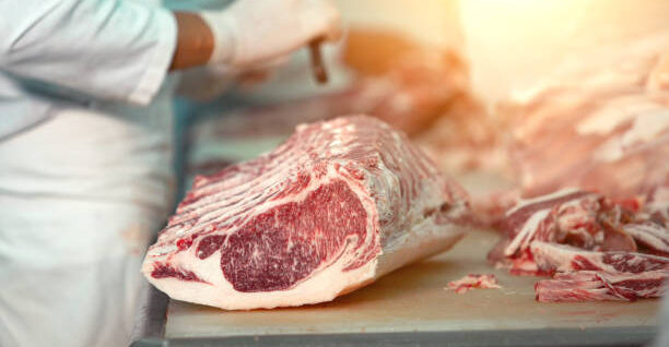
The Choice boxed beef cutout topped $400 per cwt last week and is up about $50 per cwt since the start of the year. The Choice cutout is over $400 for the first time since the 2025 highs in September. The select cutout has also surged and is at levels only surpassed by May 2020. The gap between the Choice and Select cutout has been narrow during the first few months of 2026, indicating there has not been much of a premium for Choice cattle over Select.
Boxed beef values tend to build gradually through the first quarter before accelerating in the spring and reaching a seasonal peak ahead of summer grilling season. In 2026, the cutout has surged earlier in the year as cyclical market fundamentals are outweighing typical seasonality. Cattle supplies and beef supplies are tight. When supplies are tight, wholesale prices tend to respond quickly. Additionally, buyers may be pulling some purchases forward due to expectations of tight supplies and even higher prices later this spring.
Increases in the Rib and Loin primal values since the start of the year are key contributors to the overall cutout value increase. In 2025, the Rib value ran up sharply from March to April, while the Loin value increased from March to June. This year, both primal values have been on a strong uptrend since mid-January. For producers, strong early-year boxed beef prices are supportive of fed cattle markets. Strong demand and tight supplies are supporting beef values in 2026.
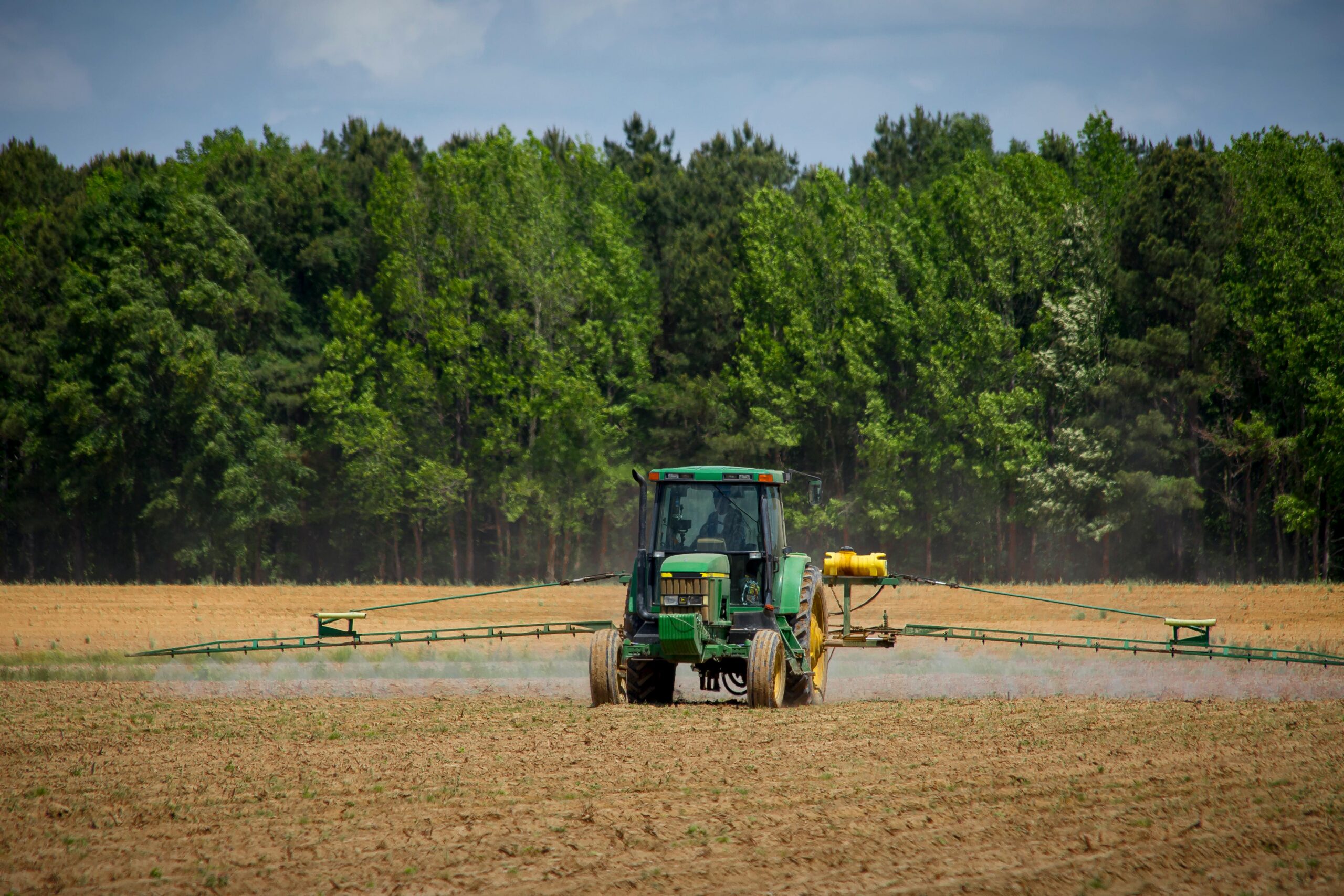
Farm equipment is a significant investment, second only to land investment for farm operations. Therefore, it is important to understand how equipment prices change over time and how that can impact a farm’s bottom line. Mississippi State University collects equipment price data every year for a large number of tractors, harvesters, implements, etc. (Gregory et al. 2025). Using that data, we can see how equipment prices have changed since 2019 and what impact that would have on costs per acre.
Figure 1 shows the purchase price for a 200-249 horsepower tractor across time. In 2019, the cost of buying this tractor was around $191,000. For 2026, the cost of this same size tractor is now $327,000, an increase of 71% (well above the rate of inflation). Also included in Figure 1 are the costs per acre for that tractor. Costs per acre are based on machine cost calculations that include labor, fuel, interest, taxes, insurance, housing, and depreciation costs. In this case, assuming that the tractor is used over 2,000 acres, the costs per acre for this tractor increased from $27.24/ac up to $41.11/ac. In other words, the same size tractor today is going to cost you $13.86/ac more than it did 7 years ago if your acreage has not changed. A producer would have to use the new tractor over 3,018 acres in order to have the same costs per acre, $27.24/ac, as it did in 2019. These per acre costs do go down on occasion, particularly when fuel prices or interest rates decline.
The purchase price and costs per acre for a cotton picker are shown in Figure 2. From 2019 to 2026, the price of a cotton picker has increased from $777,000 to $1,100,000, a 41% increase, resulting in an increase in costs per acre from $126.35/ac to $189.34/ac for the cotton picker. Lastly, the change in purchase price of a 12-row planter increased from $76,800 in 2019 to $123,600 in 2026, a 61% increase (Figure 3). This results in planter costs per acre increasing from $12.26/ac to $19.76/ac from 2019 to 2026.
Clearly, farm equipment prices have significantly increased and are likely to continue. Additionally, higher purchase costs for equipment can lead to higher financing needs and additional debt being incurred by producers. If producers are not spreading the cost of more expensive equipment across more acres, their costs of production will go up. The trend makes it harder for smaller producers to remain profitable and encourages farms to get larger and larger through economies of scale. Buying used or leasing are options to consider. Of course, some will just keep older equipment longer. Other options include equipment sharing partnerships or doing custom work for others to spread your equipment cost across more acres.