Author: Charley Martinez

  • Recent Australian Beef Import Trends

    Recent Australian Beef Import Trends

    Australian beef has become an increasingly significant presence in the U.S. import market. In 2022, Australia contributed 401.8 million pounds, roughly 12 percent of total U.S. beef imports. Australia’s share of imports has steadily grown since then, reaching 25 percent of total imports in 2025, and the trend shows no signs of reversing in 2026.

    Figure 1 illustrates Australia’s beef imports as a share of total monthly U.S. beef imports in 2025, 2026, and the five-year average from 2020 to 2024. Historically, Australian beef represented a relatively steady 13 percent to 21 percent of monthly U.S. imports. In 2025, that share climbed well above that historical norm, rising sharply through the second half of the year and peaking near 32 percent before finishing December around 31 percent. So far in 2026, the pattern has followed a similar seasonal trend, dipping in the early months before recovering, with recent months tracking above the same period in 2025. Taken together, the data makes clear that Australian beef now occupies a structurally larger share of the U.S. import market than what was considered normal just a few years ago.

    Trade Ports

    Understanding where this beef originates can also help producers and market watchers track future import flows. Australian beef exports to the U.S. move primarily through ports on Australia’s east coast. Based on the most recent available data, which captures all Australian red meat exports but is largely driven by beef, the Port of Melbourne, Victoria, accounted for 41 percent of exports. Melbourne serves as a major export gateway given the high concentration of packing facilities in the surrounding region. The Port of Brisbane, Queensland, handled 35 percent of exports and is one of Australia’s most active meat-loading ports, home to JBS Dinmore, the largest beef processing plant in the Southern Hemisphere, along with Cargill and several other major processors in the Brisbane Valley. Port Botany in Sydney, New South Wales, accounted for 19 percent of exports, while the Port of Adelaide, South Australia, and the Port of Fremantle, Western Australia, represented just 3 percent and 1 percent, respectively. The concentration of export activity through Melbourne and Brisbane reflects the infrastructure and processing capacity those regions have built to supply export markets, including an increasingly hungry U.S. import market.

    What Does This Mean? More imported beef means more competition for space in the domestic market, especially for cull cows and bulls. While the majority of imports have been lean beef trimmings for ground beef, muscle cuts are also imported, which would compete more directly with fed beef.  Imports are of particular interest now, as the U.S. cow herd sits near historic lows following years of liquidation driven by drought and high input costs. Domestic producers might have rebuilding in their plans, but rebuilding takes years and requires producer expectations of cattle prices to remain financially viable. At a time when tighter domestic beef supplies would normally support even stronger prices, the surge in Australian (and other countries’) imports is a counterweight, tempering some of the price signals U.S. producers are counting on to invest.

    Figure 1. Monthly Australia beef imports as a percentage of all US beef imports

    Source: USDA-ERS

    Recommended citation format: Martinez, Charley. “Recent Australian Beef Import Trends.” Southern Ag Today 6(36.2). September 1, 2026. Permalink
  • Check in on Current Non-Real Estate Farm Debt

    Check in on Current Non-Real Estate Farm Debt

    Authors: Charley Martinez, Mason Collins, and Eli Mundy

    As mentioned in previous Southern Ag Today (SAT) articles (Martinez and Ferguson 2022, Martinez 2023), monitoring Non-Real Estate Farm Debt provides insight into debt health. At the time of this article, planting season has begun or is in full swing for others, input prices have increased over the last few weeks, and livestock prices have remained at high levels. Last month, the Federal Financial Institutions Examination Council released its most recent Call Reports, which provided insights into the final quarter of 2025. As a refresher, every commercial bank in the U.S. submits its quarterly Reports of Condition and Income, which are known as call reports. Within these call reports are totals of agricultural loans and the status (on time or late) of the loans. Figure 1 displays the total loan volume (yellow line) and loan volume for three late categories (30-89 days late, 90+ days late, non-accrual) for the last 12 quarters (3 years). The totals are for all the Southern Ag Today States. 

    In the fourth quarter of 2025, total non‑real estate loans (yellow line) continued to trend upward overall and was 4% higher compared to 2024 Q4. Non-accrual (blue line) loans remained elevated at the 2025 Q3 levels, and increased 172% from 2024 Q4. Loans that are 90+ days late (grey line) remained about the same as 2024 Q4, and decreased 3%. Last year, the most concerning statistics were the loans that were 30-89 days late (orange line), which increased to $108.9 million in Q1 in the SAT states. By the end of the year, total loan amounts in this category decreased to $49.6 million, but it seems the decline was the result of debt moving to the non-accrual category by Q4 of 2025. While this loan type decreased from Q1, the amount increased by 35% compared to 2024 Q4. Due to the varying size of states, measuring the percentage of 30-89 days late loans compared to total loan volume is a good way to compare the SAT states and the impacts of these bad loan types. In 2025 Q4, the quarterly average of 30-89 days late loans to total loan volume was 0.3% (which is stable), with the highest being  Kentucky (0.8%), North Carolina (0.5%), and Louisiana (0.4%). When comparing the percentage of total late debt (non-accrual, 30-89 days late, and 90+ days late) relative to total loan volume, the quarterly average was 0.9%. Alabama (3.1%), Georgia (2.4%), Louisiana (1.8%), Mississippi (1.2%), and Arkansas (1.1%) were the only states above the SAT average. North Carolina and South Carolina were the only two states below 1%. 

    Taking a broad view, the 2025 fourth‑quarter bank reports give a useful snapshot of farm debt conditions following a difficult profitability year for many row‑crop operations and a strong revenue year for livestock producers across the SAT states. The reports show that financial condition remains stable in several states, but there are also early warning signs in others that warrant close attention. Recent improvements in row‑crop prices offer some potential relief for operating debt in 2026, though margins remain tight. Government payments will also be an important factor this year; ARC and PLC payments are expected again for the current crop year, though they will not be received until October 2026, and should help reduce some problem loan balances. In the meantime, producers should closely monitor working capital, manage short‑term debt carefully, and continue the sound production, marketing, and risk‑management practices they already have in place. Overall, while reliance on non‑real estate credit has increased, rising input costs, higher interest rates, and income variability are placing added pressure on farm finances, making proactive financial management especially important in the months ahead.

    Figure 1. Non-Real Estate Farm Debt from 2023 Q1- 2025 Q4

    Source: Federal Financial Institutions Examination Council

    References

    Martinez, Charley, and Haylee Ferguson. “Current Non-Real Estate Farm Debt“. Southern Ag Today 2(30.3). July 20, 2022. Permalink


    Martinez, Charley, Mason Collins, and Eli Mundy. “Check in on Current Non-Real Estate Farm Debt.” Southern Ag Today 6(21.1). May 18, 2026. Permalink

  • Price Relationships of Beef X Dairy Calves and Dairy Calves

    Price Relationships of Beef X Dairy Calves and Dairy Calves

    Authors: Charley Martinez, Parker Wyatt, and Eli Mundy

    Over the last few years, the Beef X Dairy (BxD) markets have gained attention due to the rise in BxD prices. Day-old calves (80-90 pounds) have gone from $50 per head a few years back to recent Pennsylvania auction data showing 80-89 pounds BxD calves averaged $1706.21 per head for the week ending March 21st. A question that has been asked recently is centered around the value of purebred dairy calves compared to BxD calves. For the same week, 80-89 pound purebred dairy calves averaged $1329.60 per head, a difference of $376.60. This SAT examines the premium over time for BxD calves over purebred dairy calves. 

    The United States Department of Agriculture’s (USDA) weekly New Holland Pennsylvania market report currently provides the most extensive and consistent information regarding the price of BxD and purebred dairy calves. Very few markets report BxD calves separately, and there may be variation in local prices influenced by regional differences in demand, transportation cost, and buyer composition. Figure 1 shows the price premium received for BxD calves over purebred dairy calves at the Pennsylvania market for the previous 5-year average (2020-2024), 2025, and 2026.  

    Figure 1. Monthly Premium for BxD Calves Over Purebred Dairy Calves ($/head), New Holland, PA.

    Data from USDA-AMS

    The chart shows a consistent premium per head for BxD calves relative to purebred dairy calves with increased premiums during August through October. During 2020–2024 (thick red line), the average premium ranged from about $130 (first quarter) to $200 per head (August-October). In 2025 (dotted line), the premium was notably higher than the previous 5-year average, beginning the year at approximately $255 per head in January, climbing through the spring, and reaching its highest levels of about $450–$470 per head in early fall, before declining toward year‑end. In 2026 (thin solid blue line), there has been an even larger premium than last year, approximately $340 in January and over $420 per head by February. This suggests an exceptionally strong relative demand for BxD calves compared to dairy calves during that period. 

    With no clear signs of increases in the beef calf crop, the premiums for BxD calves can be expected to remain strong or continue to increase. These premiums reflect tight supplies of feeder cattle and a willingness from feedlot operators to pay for calves that offer improved feed efficiency, growth performance, and carcass characteristics relative to purebred dairy calves. This raises a few important questions: how high can the premium go, and what happens when traditional beef cattle numbers begin to rise? If the beef herd expansion is relatively gradual, BxD calves may retain a meaningful premium and a strong role in the supply chain. Conversely, rapid rebuilding of the beef herd could result in a faster narrowing of the price differential, particularly if feedlot operators shift back quickly to traditional beef calves. Ultimately, the long-run trajectory of BxD premiums will hinge on the rate of supply growth, their ability to compete with traditional beef calves on feedlot efficiency, and downstream demand for beef. 


    Martinez, Charley, Parker Wyatt, and Eli Mundy. “Price Relationships of Beef X Dairy Calves and Dairy Calves.” Southern Ag Today 6(14.2). March 31, 2026. Permalink

  • The Impact of Tyson’s Closure on Beef Slaughter Capacity Utilization

    The Impact of Tyson’s Closure on Beef Slaughter Capacity Utilization

    This year, there have been several Southern Ag Today articles discussing the impacts of tight fed cattle supplies on prices, cattle on feed, slaughter weights, and total beef production (Anderson 2025a, Anderson 2025b, Maples 2025). On November 21, Tyson announced that they would be closing their Lexington, Nebraska plant in January 2026. Following the announcement, there have been a lot of questions revolving around the impact of the closure on national slaughter capacity utilization (CU). 

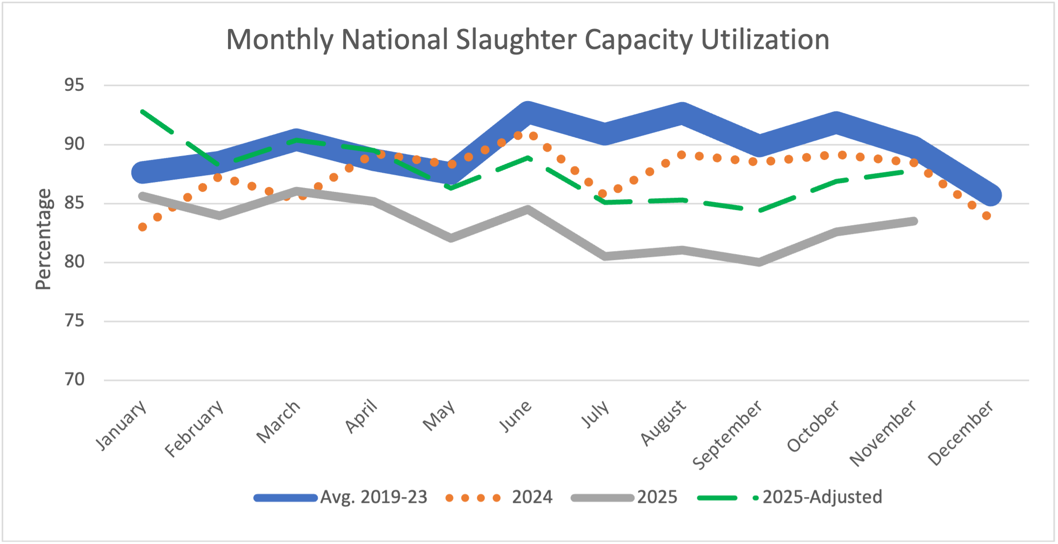
    The Lexington, Nebraska plant had an approximate daily capacity of 5,000 head. That equates to approximately 20% of Tyson’s daily capacity (25,800 head/day) as a company. In Martinez et al. (2023), we showed a measure of national slaughter capacity utilization, which measures the ratio of operational cattle slaughter capacity over total physical capacity. To estimate the impact of the closure on the national CU, we use 2025’s monthly slaughter with an adjusted 2025 slaughter CU. The adjusted CU is simply adjusting the national CU with the daily 5,000 head taken out. Figure 1 displays the monthly national federally inspected (FI) slaughter capacity utilization with the previous 5-year average (thick blue line), 2024 (orange dotted line), 2025 (grey thin line), and 2025-Adjusted (green dashed line). 

    Figure 1. Monthly National Federally Inspected Slaughter Capacity Utilization

    The adjusted capacity utilization is closer to the previous 5-year average. Evaluating data through November, the average for the 5-year average was 90.1% while the 2025 and 2025-adjusted average through November are 83.1% and 87.7%, respectively. In November, slaughter capacity utilization averaged 83.5%, which was lower than November 2024 (88.4%), the previous 5-year average (89.8%), and the 2025-adjusted (87.8%).Overall, 2025 has seen declining fed cattle numbers in the cattle on feed reports and higher fed cattle prices, leading to low or negative packer margins. While the supply chain is offsetting tight cattle supplies with larger carcasses, the closure of the Lexington plant certainly signals there is excess capacity at this time. This is the first large scale plant to close since 2013, when Cargill closed their Plainview, TX plant, which was also during a time when cattle supplies were tight.  There have been reports that Tyson is looking to buy that Plainview plant. Additionally, there are some plants that are reported to come online in 2026 and 2027. It is fair to question if the adjusted capacity utilization is a new norm, or simply a short run adjustment by the supply chain.

    References

    Anderson, David. “Fewer Marketings, Tighter Beef Supplies.” Southern Ag Today 5(26.2). June 24, 2025. 

    Anderson, David. “Working Less on Friday!” Southern Ag Today 5(21.2). May 20, 2025.

    Maples, Josh. “Cattle Prices Hit New Highs and Carcass Grading Trends Over Time.” Southern Ag Today 5(19.2). May 6, 2025.

    Martinez, C., Li, P., Boyer, C. N., Yu, T. E., & Maples, J. G. (2023). Beef price spread relationship with processing capacity utilization. Journal of the Agricultural and Applied Economics Association.https://onlinelibrary.wiley.com/doi/full/10.1002/jaa2.48


    Martinez, Charley, and Parker Wyatt. “The Impact of Tyson’s Closure on Beef Slaughter Capacity Utilization.” Southern Ag Today 5(49.2). December 2, 2025. Permalink

  • A Check in on the Beef Cutout

    A Check in on the Beef Cutout

    The current government shutdown has caused many weekly and monthly reports to not be published. However, USDA-AMS is still generating their daily and weekly reports. The beef industry knows that tight supplies have led to increased price movements over the last couple of years, but beef demand has become a hot topic as of late due to retail beef prices continuing to set all-time highs every month. These market movements have led to a common question, “could demand be decreasing and that’s why the cutout has been decreasing?” One data series that offers valuable insight into the intersection of beef supply and demand is the cutout value.

    Figure 1 shows the weekly choice cutout value for this year, last year, and the previous 5-year average. In mid-September, the choice cutout peaked at $413.60/cwt, has steadily decreased each week, and finished last week at $365.25/cwt. This decline is somewhat expected due to seasonality trends. However, last week’s price was $56.82/cwt (18.4%) and $113.57/cwt (45.12%) higher than last year and the previous 5-year average for the same week. Even though the market has experienced peaks and recent declines in the choice cutout value, year-over-year demand indices suggest historically strong demand as consumers pay higher prices for the smaller amounts of beef available.  

    Consumers make choices not only between cuts of beef but also grades of beef. Figure 2 shows the monthly cutout values by grade for the last 12 months. Since March of this year, each cutout grade has trended upward through September. Interestingly, the last two months have also had increasing spreads between prime and all other grades. To the question posed in the introduction paragraph, there is little data to suggest weakening demand. Tight beef supplies are driving prices higher and consumer demand is holding strong. Consumers will eat less beef overall in 2025 due to less availability, but the higher prices will allocate the various grades and cuts of beef to consumers.  

    Figure 1. Weekly Choice Cutout Value

    Figure 2. Monthly Graded Cutout Values for the previous 12 months


    Martinez, Charley, Parker Wyatt, and David Eli Mundy. “A Check in on the Beef Cutout.” Southern Ag Today 5(42.2). October 14, 2025. Permalink