Author: Hence Duncan

  • Revenue Protection Weighted Average Coverage Levels by County and Crop

    Revenue Protection Weighted Average Coverage Levels by County and Crop

    Producers make several important marketing and risk management decisions throughout the year. One of the most important decisions is the choice of coverage levels when purchasing crop insurance. Revenue Protection (RP) – by far the most popular plan of insurance – provides an indemnity if realized revenue (combination of yield and price) drops below the guarantee (or a percent of expected revenue) for the insured unit. RP coverage levels range from 50% to 85% of expected revenue, increasing in 5% increments. Producers must weigh the choice of varying RP coverage levels against the changes in premium costs. Premium costs vary and consider factors such as the risk of loss for the insured crop in the specific county, coverage level, insurance product purchased, and production practices. This article examines the weighted average coverage level (WACL) by county and crop from 2011-2022 for corn, cotton, soybean, wheat, and peanut RP insurance plans. RP insurance plans from 2011 to 2022 covered 88% of all insured acres for corn, cotton, peanuts, soybeans, and wheat (USDA Summary of Business). The WACL is calculated as RP coverage level multiplied by acres insured for the coverage level divided by total RP acres insured for each county crop and year.

    Corn

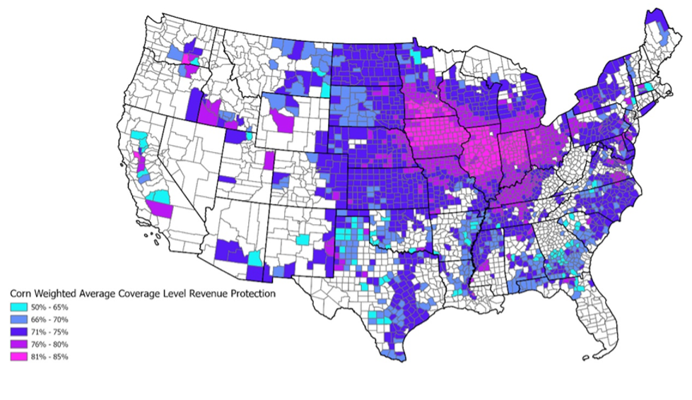
    The Corn Belt states of Indiana, Illinois, and Iowa show most counties have a WACL of 81% to 85%, indicating higher insurance coverage purchases. Most counties in North Dakota, South Dakota, Nebraska, and Kansas exhibit a WACL of 71% or greater. However, there is more variability in the southern and eastern states, with coverage levels generally lower than in the Midwest.

    Figure 1. Corn Acre-Weighted Average Coverage Level Revenue Protection 2011-2022

    Data Source: USDA RMA Summary of Business

    Cotton

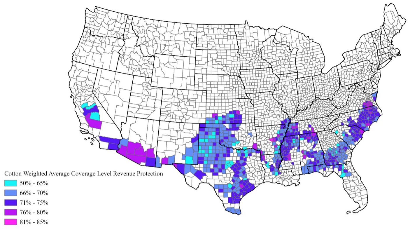
    Southern Arizona has a concentration of 76% to 80% WACLs for cotton, while the majority of Western Oklahoma and Texas counties have a WACL for cotton of 66%-70%. The rest of the south’s cotton production is concentrated along the Mississippi River, the east coast, South Georgia, and South Alabama with a 71-75% WACL being the most prominent coverage level. Nationally, there are very few counties with a WACL above 80% for cotton.

    Figure 2. Upland Cotton Acre-Weighted Average Coverage Level Revenue Protection 2011-2022
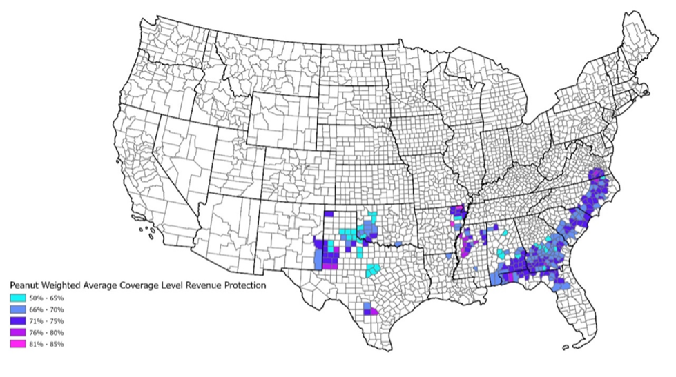
    Data Source: USDA RMA Summary of Business

    Peanuts

    The southern regions of Alabama, Georgia, and the eastern Carolinas show a WACL between 66% and 75%. About half of the counties in Northeast Arkansas and Northwest Mississippi have a WACL of 76% or higher. The counties along the border of Western Oklahoma and Texas have lower WACLs, while those along the border of West Texas and Eastern New Mexico mainly have WACLs of 71% or higher. Like cotton, peanuts have few counties with WACLs that exceed 80% – fewer than twenty counties have WACLs greater than 76%. 

    Figure 3. Peanuts Acre-Weighted Average Coverage Level Revenue Protection 2011-2022
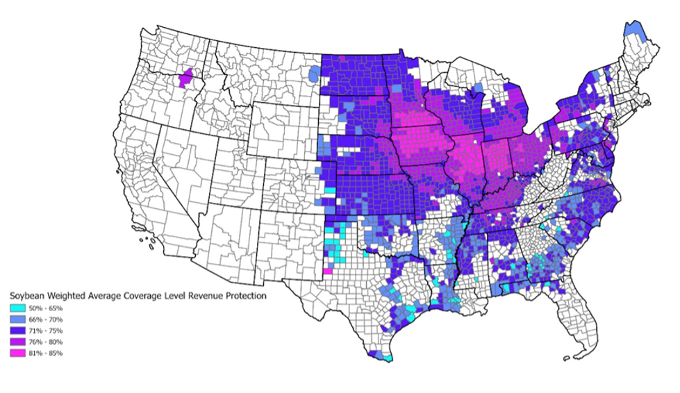
    Data Source: USDA RMA Summary of Business

    Soybeans

    Trends for soybeans mirror those for corn, with counties in Ohio, Indiana, Illinois, Iowa, and Kentucky showing WACLs of 76% or higher, with many reaching 81% or higher. From North Dakota to Kansas, counties have WACLs of 71% or better. In the southern states, the WACL varies significantly.

    Figure 4. Soybeans Acre-Weighted Average Coverage Level Revenue Protection 2011-2022
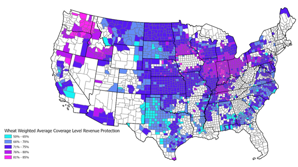
    Data Source: USDA RMA Summary of Business

    Wheat

    Northwestern states and parts of the Midwest exhibit WACLs of 76% or greater. In Texas, many counties show lower WACLs, ranging from 50% to 70%. Wheat production varies by season (spring or winter) and type (hard, soft, and durum). Wheat production in the northwestern states is typically soft spring wheat, whereas Texas wheat is mostly hard red winter wheat that produces lower yields than soft wheat. 

    Figure 5. Wheat Acre-Weighted Average Coverage Level Revenue Protection 2011-2022

    Data Source: USDA RMA Summary of Business

    Since the early 1990s, buyup coverage levels for crop insurance have trended higher (Smith, 2015). From 2011 to 2022, across commodities there is greater variability in WACLs in the South than the Midwest and Northern Plains. Variability in WACLs by crop and region highlights differences in risk levels, risk preferences, insurance premiums, and production costs. Regions with higher WACLs often have more consistent yields; regions with lower WACLs typically face higher premium costs due to greater production variability. Understanding trade-offs in risk and premium cost can help producers determine the correct RP insurance coverage level to meet their specific risk management needs.

    References and Resources:

    Biram, H.D. 2024. The Fundamentals of Federal Crop Insurance, University of Arkansas. Link

    Smith, S.A., J. Outlaw, and R. Tufts. 2015. Surviving the Farm Economy Downturn. Chapter 10. Crop Insurance: Basic Producer Considerations. https://afpc.tamu.edu/extension/resources/downturn-book/.

    USDA Risk Management Agency. Summary of Business. https://www.rma.usda.gov/SummaryOfBusiness


    Duncan, Hence, and Aaron Smith. “Revenue Protection Weighted Average Coverage Levels by County and Crop.Southern Ag Today 4(28.1). July 8, 2024. Permalink

  • Corn and Cotton Prevented Planting Decisions 

    Corn and Cotton Prevented Planting Decisions 

    From 2019 to 2023, 4.6 million corn acres and 1.4 million cotton acres in the 13-state southeast region were prevented from planting (Table 1; USDA-FSA).

    Table 1. Corn and Cotton Prevented Planted Acres for 13 Southern States, 2019-2023

    Source: USDA Farm Service Agency Crop Acreage Data

    Prevented planting is a provision covered by the United States (US) Federal Crop Insurance Program that compensates producers for losses from delayed planting or not being able to plant an eligible crop within that crop’s region-specific planting period. Under the prevented planting provision, revenue protection (RP), revenue protection with harvest price exclusion (RP-HPE), and yield protection (YP) crop insurance pay producers an indemnity if they are impeded from planting an insured crop by a designated final planting date, or within any applicable late planting period.[1] If a producer – who purchased a qualifying policy – is unable to plant by the final planting date, there are four options: 

    1. Plant the insured crop in the late planting period with reduced insurance. For most crops, the production guarantee[2] decreases one percent per day, for each day of delay after the final plant date until the crop is planted or the end of the late planting period. Late planting periods vary by crop and area.

    2. Take the prevented planting payment, based on the applicable prevented planting factor, and leave ground fallow or plant a summer cover crop after the late planting period. Summer cover crops cannot be harvested or grazed before November 1. 

    3. Receive 35% of the prevented planting payment for the original crop and switch to an uninsured second crop.

    4. Forgo the prevented planting payment for the first crop and plant an insured second crop.

    Figure 2. Corn Prevented Planting Decision Tool Results

    Source: University of Tennessee Prevented Planting Decision Aid
    Projected results are dependent on user specified variables and are displayed for educational purposes only. Actual results may vary based on market conditions and individual circumstances. 

    The tool depicted in Figure 2 charts the average net returns across all four prevented planting options, aiding producers in their prevented planting decisions.  Projected net returns are operation specific and will change by commodity market prices, planting costs, average production history (APH), coverage level, and insurance premium costs. Changing each variable to fit an operation allows producers to quantify the impacts of each prevented plant decision.  

    The example in Figure 2 depicts a corn-soybean prevented plant scenario where taking 35% of the full prevented planting payment and planting uninsured soybeans provides the highest projected net returns from June 4th to July 2nd (yellow line in figure 2). After July 2nd, taking the full prevented planting payment provides higher net returns due to the yield losses from later season beans (blue line in Figure 2). It is worth noting that planting an uninsured second crop and taking 35% of the full prevented planting payment is a riskier decision than taking the full prevented planting payment. Regardless of date, planting insured beans or late planted corn are projected lower net return decisions in this scenario. Net returns by day of year are based on Tennessee data and may vary between states. 

    Prevented planting decisions can have large financial impacts on crop producer profitability. In our scenario, late planted corn could even result in a net loss. The prevented plant decision can be quantified by utilizing a prevented planting decision tool to maximize net returns at the farm level. 


    [1]The final planting date is the last day to plant an insured crop and be eligible for full coverage. The late planting period begins the day after the final planting date and ends 25 days after the final planting date. Final and late planting periods vary by crop and region.

    [2] The production guarantee is the guaranteed revenue or yield offered by the crop insurance policy. For an RP policy, the guarantee is calculated by multiplying the insurance price by actual production history (APH) yield, which is a 4-to-10-year trend adjusted average yield used for future crop insurance purchases, by insurance coverage level.

    References

    University of Tennessee Prevented Planting Decision Aid. Available at https://arec.tennessee.edu/prevented-planting-decision-aids/  

    University of Tennessee Field Crop Budgets. 2024. Accessed at: https://arec.tennessee.edu/extension/budgets/

    USDA Farm Service Agency Crop Acreage Data. 2019-2023. Accessed at https://www.fsa.usda.gov/news-room/efoia/electronic-reading-room/frequently-requested-information/crop-acreage-data/index

    USDA Risk Management Agency. Prevented Planting Insurance Provisions Flood. Accessed at: https://www.rma.usda.gov/en/Fact-Sheets/National-Fact-Sheets/Prevented-Planting-Insurance-Provisions-Flood

    USDA Risk Management Agency. Prevented Planting Insurance Provisions Drought. Accessed at: https://www.rma.usda.gov/en/Fact-Sheets/National-Fact-Sheets/Prevented-Planting-Insurance-Provisions-Drought

    USDA Risk Management Agency. Prevented Planting. Accessed at: https://www.rma.usda.gov/en/Topics/Prevented-Planting

    Duncan, Hence, Chris Boyer, and Aaron Smith. “Corn and Cotton Prevented Planting Decisions.Southern Ag Today 4(15.1). April 8, 2024. Permalink

  • Bridging the Price Risk Gap

    Bridging the Price Risk Gap

    At the end of the calendar year, many producers prepay for inputs to reduce taxes and potentially avoid higher prices in the spring. To prevent the risk of profit margin reductions (from a decline in commodity prices), producers may want to consider obtaining downside price protection for a portion of their anticipated 2024 production at the same time as inputs are purchased. One strategy is purchasing put options on the yield required to pay for the input purchased, and carrying the put option position until the projected crop insurance price is determined.

    Table 1 shows a simple budget for Tennessee corn production (target yield of 180 bu/acre), and the number of bushels of production required to cover the specified expense at different corn prices. This is computed as the cost of the production input per acre divided by the harvest price.  For example, a fertilizer expense of $181.80/acre would require 40.4 bu/acre to cover the fertilizer expense at a corn price of $4.50/bu, 38.3 bu/acre at a corn price of $4.75/bu, or 36.4 bu/acre at a corn price of $5.00/bu. A producer can mitigate financial risk by using put options to cover the amount of production needed to cover that input cost, thus bridging the price risk gap until crop insurance prices and revenue protection are determined. 

    A producer with 260 acres of corn, seeking to set a futures price floor at $4.75/bu and provide sufficient price protection on the bushels needed to pay the fertilizer expense, could purchase two put options (5,000 bushels each covering 260 acres x 38.3 bu/acre = 9,958 bushels). On November 21st a $5.20 December 2024 corn put option could be purchased for 45 cents, setting a $4.75 futures floor. The put option could be carried until March 1, at which time projected crop insurance prices are established and revenue protection for the upcoming crop are determined. At that time, the option purchaser can evaluate the price protection their crop insurance provides and decide to maintain the put option position or exit. If the December corn futures contract is below $4.75, the purchaser can maintain the put option position for additional price protection or exercise the option for a financial gain. If the December corn contract is above $4.75, the purchaser can maintain the position or exit the put option position and recoup a portion of the premium based on the time value remaining.  

    Producers should examine times during the year when they are exposed to price and financial risk and seek strategies to mitigate those risks. Using put options can be an effective tool to remove some price risk when prepaying for fertilizer, and other inputs, until crop insurance prices and revenue protection are determined. 

    Table 1. Tennessee Corn Budget for 2024 and Number of Bushels to Cover a Specified Expense at Three Corn Prices

    References:

    Barchart.com. December 2024 Corn Options Prices. Accessed at:  https://www.barchart.com/futures/quotes/ZCZ24/options   University of Tennessee Field Crop Budgets – https://arec.tennessee.edu/extension/budgets/

  • Soybean Indemnity Payments for Wildlife Damage

    Soybean Indemnity Payments for Wildlife Damage

    Often, we think of crop loss being caused by weather, such as drought or excess moisture. However, a lesser quantified, but growing, cause of loss for crops in the southeast United States is wildlife damage. The most common causes of wildlife damage in soybeans are deer and hogs. Wildlife damage can be quantified when crop yield is damaged to a level that triggers an indemnity payment. Using the USDA RMA cause of loss data, Figure 1 shows the county map of soybean indemnity payments due to wildlife damage from 2011 to 2022; Figure 2 shows the percent of total soybean wildlife indemnities as a percent of total insured liability for soybeans by county. Mississippi received the most payments totaling $6.54 million, and Arkansas received the least number of payments, totaling $1.1 million. Tennessee was second with $5.65 million and Kentucky was third with $5.5 million. Missouri received $4.3 million, and Alabama received $2.4 million. 

    We also show the annual losses to wildlife damage for soybeans in the seven states combined (Missouri, Kentucky, Arkansas, Tennessee, Mississippi, Alabama, and Georgia) from 2011 to 2022 (Figure 3). Indemnity payments due to wildlife damage to soybeans in 2022 were approximately $4.8 million, which is a 487% increase from 2011. Between 2011 and 2022, in these seven southeastern states, a total of 250,818 soybean acres received an indemnity payment due to wildlife damage. Figure 3 also shows the percentage of total soybean indemnity payments caused by wildlife damage (orange line). These indemnities due to wildlife losses are a small percentage of the total soybean crop insurance losses but have increased since 2011. 

    It should be noted that the total indemnity payments received do not capture the total loss of wildlife damage in soybean fields. Before an indemnity payment is made, the actual revenue or yield must be below the crop insurance yield or revenue guarantee for the insured unit. Also, damage to uninsured acres would not be accounted for in the data. Further, some losses due to wildlife may be being attributed to another cause that also impacted the farm (e.g. drought or excess moisture). As such, indemnities paid due to wildlife losses in soybeans represent only a portion of actual producer losses. In the seven-state region, state average soybean crop insurance coverage levels for 2022 (2011-2022 average) were: Alabama 72.1% (71.6%), Arkansas 63% (62.2%), Georgia 67.6% (66.8%), Kentucky 76.1% (76.2%), Missouri 73.2% (73.0%), Mississippi 69% (69.2%), and Tennessee 72% (72.2%).

    We note that some states and counties allow for nuisance hunting permits out of season to control deer and hog damage to crops. It might be of interest to check with your local game warden to determine if this is an option for your farm.  

    Figure 1. Soybean Indemnity Payment Map for Wildlife Damage Cause of Loss for Missouri, Kentucky, Arkansas, Tennessee, Mississippi, Alabama, and Georgia from 2011 to 2022

    Figure 2. Percent of Wildlife Damage Cause of Loss as a Percent of Total Insured Liability for Missouri, Kentucky, Arkansas, Tennessee, Mississippi, Alabama, and Georgia from 2011 to 2022

    Figure 3. Soybean Wildlife Indemnity Payments for Missouri, Kentucky, Arkansas, Tennessee, Mississippi, Alabama, and Georgia and Percent of Total Soybean Indemnity Payments Caused by Wildlife Damage by Year from 2011 to 2022

    References

    U.S. Department of Agriculture – Risk Management Agency. Cause of Loss Historical Data Files 2011-2022. Accessed at https://www.rma.usda.gov/SummaryOfBusiness/CauseOfLoss

    Duncan, Hence, Chris Boyer, and Aaron Smith. “Soybean Indemnity Payments for Wildlife Damage.Southern Ag Today 3(29.1). July 17, 2023. Permalink

  • Estimating the Cost of a Grain Bagging System

    Estimating the Cost of a Grain Bagging System

    Storage can be a valuable risk management and marketing tool for Southern corn producers. Storage allows producers to reduce harvest delays, avoid seasonal price lows, expand the marketing window, and harvest grain at higher moisture – if drying or aeration is available. There are two main options to store grain: grain bins or grain bags. This article provides an overview of the benefits, ownership costs, and operating costs for a grain bagging system.

    Benefits

    Labor continues to be a major challenge for agricultural producers. One of the primary benefits to using a bag system is the ability to reduce harvest labor requirements, particularly trucking. Storing corn at the edge of the field reduces the number of trucks required to keep combines running, avoids long lines at elevators and barge points, and distributes hauling to terminal markets during times of the year when labor is more readily available. Additionally, the ability to harvest a crop quickly reduces the risk of losses due to adverse weather. Extending the marketing interval allows producers to benefit from post-harvest price rallies. For example, in Memphis Tennessee, the ten-year average corn price was 70 cents higher in March/April compared to the harvest low. Mid-south producers that have cotton in their crop rotation can use bagging systems to modify annual storage availability, thus avoiding capital investment in permanent grain storage infrastructure when planted acreage varies year-to-year.

    Ownership Costs

    A bagging system requires capital investment in a loader, unloader, and tractor. This equipment is in addition to grain carts/trucks to transport grain from the combine to bagger. Purchase prices vary however many loaders can be obtained for less than $50,000. Bag unloaders will also cost around $50,000. Most operations will have access to a tractor that can be utilized in a bagging system, however this cost should also be included. Cost of ownership will vary for each operation; however, cost estimates should include capital recovery (depreciation + interest), taxes, insurance, and housing (TIH). For example, assuming an interest rate of 6.5% and TIH of 2.0% of the equipment value, estimated ownership costs for 100,000 bushels of storage is approximately 14 cents/bushel. Storing more bushels will distribute fixed costs lowering the ownership cost per bushel. 

    Operating Costs

    Operating costs vary by system; however, producers should consider site preparation, purchase price of storage bags, labor (loading, unloading, and monitoring), insecticides, sensors, bag disposal, and machinery expenses (fuel, repair and maintenance). Additionally, producers should account for potential storage loss/risk. Wildlife damage, insect and rodent infestation, weather, and damage from humans present a risk for storage losses. Estimated operating costs based on the assumptions below in Table 1 are 17-22 cents per bushel. Costs are highly variable so producers are encouraged to estimate costs based on operation specific variables and assumptions.

    Bagging systems may be a cost-effective method to store grain for Mid-south producers. Producers are encouraged to weigh the advantages and disadvantages of permanent storage (bin) and temporary storage (bag) systems to determine which system is best for their operation. Additionally, comparing ownership and operating costs with seasonal corn prices in your area will assist in determining if investment in storage is financially beneficial for your operation.

    Table 1. Example: Operating Cost Assumptions

    ValueUnit
    Bag Size16,000bu
    Bag Price$1,100$/bag
    Labor Rate$22,000$/hr
    Diesel Price$6.00$/gallon
    Interest Rate (Operating)6.5%%
    Repair and Maintenance5.0%% of purchase price

    Resources:

    Estimating Costs for Grain Storage: Bags and Bins- https://extension.tennessee.edu/publications/Documents/W1060.pdf

    Spreadsheet: https://arec.tennessee.edu/grain-bag-and-bin-storage/


    Duncan, Hence, and S. Aaron Smith. “Estimating the Cost of a Grain Bagging System.” Southern Ag Today 2(31.3). July 27, 2022. Permalink