Author: R. Jamey Menard

U.S. agricultural producers use hired farm labor for field crops, livestock, and nursery operations, for grading and sorting of agricultural products, for supervisory roles, and other areas. According to USDA’s Economic Research Service (ERS), mechanization led to greater productivity and a reduction in the need for labor, both self-employed farm operators (including family members) and hired workers, from 1950 to 1990. Since 1990, however, U.S. employment of agricultural workers has stabilized. For the 1950 to 1990 period, labor from self-employed and family members experienced a greater decline (74 percent) than hired farm labor (51 percent reduction). Even though hired farm labor comprises only one percent of all U.S. wage and salary workers, hired labor is important for agriculture to succeed (USDA/ERS, 2025).

Table 1 contains census of agriculture data for the number of hired farm laborers and farms with hired farm labor from 2012 to 2022, along with the ten-year average change for the southern states. There should be no surprise that all southern states have witnessed a decrease in both workers and farms with hired farm labor (for Maryland, the number of farm workers is essentially flat, but farms with hired labor are declining). Kentucky leads in the loss of hired farm labor over the ten-year average at -23.2%, followed by Oklahoma (-18.1%). Kentucky also leads in the decrease in the number of farms with hired farm labor at -18.7%, followed by Mississippi (-16.6%). For Kentucky during this timeframe, there was a shift away from tobacco production, a highly labor-intensive crop. Florida and Georgia have lost the fewest workers as measured by the ten-year average (USDA/NASS, 2025a). The prevailing reasons for the decrease in hired farm labor are the aging of the farm workforce, the lack of new immigrants entering agriculture, the displacement of labor by technology and machinery, costs, a lack of interest, and a preference for a better life-work balance.

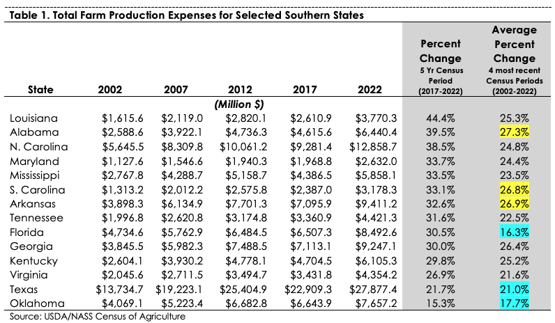
The 2022 agriculture census indicates that hired farm labor ranked third in a ranking of production expenses for southern states, preceded by feed purchases and livestock and poultry purchased/leased (see Menard SAT “Census of Agriculture Production Expenses for Southern States, 11/11/24). For all farms, data from the most recent agriculture census indicate that wages and salaries plus contract labor are 12 percent of production expenses. However, this percentage increases to 42 percent for greenhouse and nursery operations and 40 percent for fruit and tree nut operations. For immigrant labor costs in dairies and nurseries, costs as a share of gross revenues are near their 20-year highs. Hired farm labor wages vary by state and farm region. For 2024, the hourly wage rates for hired farm labor in the southern states range from $15.25 (Arkansas, Louisiana, and Mississippi) to $19.15 per hour (Maryland). For that same timeframe, hired farm labor ranges from $14.86 to $18.13 per hour for crop operations and $14.73 to $17.51 per hour for livestock operations (USDA/ERS, 2025; USDA/NASS 2025a & 2025b).

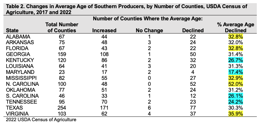
For 2022, the most common agriculture operation type for each state where hired farm labor was utilized is indicated in Table 2. The table also provides information for each state on the operation type having the largest hired farm labor production costs. For example, beef cattle (NAICS 112111) farming was the most common operation type for hired farm labor in Alabama, Kentucky, Oklahoma, Tennessee, and Texas. Greenhouse, nursery, and floriculture production operations had the highest hired farm labor production costs for Alabama, Florida, Maryland, North Carolina, South Carolina, Tennessee, and Virginia.

There are a couple of interesting trends moving forward that may affect southern states and the use of hired farm labor.  Long-distance migrations from home to work are declining —farmworkers are more settled.  Fewer farmworkers are pursuing the seasonal follow-the-crop migration. Also, women as farmworkers is an increasing trend. (USDA/ERS, 2025; USDA/NASS, 2025a). 

Reference

USDA Economic Research Service (ERS). 2025. “Farm Labor.” Available at https://www.ers.usda.gov/topics/ farm-economy/farm-labor.

USDA National Agricultural Statistical Service (NASS). 2025a. Census of Agriculture Reports. Available at https://www.nass.usda.gov/AgCensus/index.php.

USDA National Agricultural Statistical Service (NASS). 2025b. “Quick Stats.” Available at https://quickstats.nass.usda.gov/

Menard, R. Jamey. “Hired Farm Labor Trends.” Southern Ag Today 5(34.1). August 18, 2025. Permalink

The most recent agriculture Census defines total farm production expenses as “expenses provided by producers, partners, landlords (excluding property taxes), and production contractors for the farm business” (USDA/NASS, 2024). Based on Census data from 2017 to 2022, all southern states experienced higher overall production expenses (Table 1 in descending order based on change from 2017 to 2022). For 2017 to 2022, the top three states with the highest increases in production expenses were Louisiana (44.4% increase), Alabama (39.5%), and North Carolina (38.5%). The lowest were Oklahoma (15.35 increase), Texas (21.7%), and Virginia (21.6%). For the twenty-year timeframe 2002 to 2022, Alabama, Arkansas, and South Carolina had the largest production expense increases (yellow highlight), whereas Florida, Oklahoma, and Texas had the lowest (blue highlight).

Total farm production expenses in the Census are comprised of the following categories 1) fertilizer, lime, and soil conditioners, 2) chemicals, 3) seed, plants, vines, & trees, 4) livestock & poultry, 5) feed, 6) gasoline, fuels, and oils, 7)utilities, 8) repairs, supplies, & maintenance costs, 9) hired farm labor, 10) contract labor, 11) custom work & custom hauling, 12) cash rent for land, buildings, & grazing fees, 13) rent & lease expenses for machinery, equipment, and farm share of vehicles, 14) interest expense, 15) property taxes, 16) medical supplies, veterinary, & custom services for livestock, and 17) all other production expenses (defined as storage and warehousing, marketing and ginning expenses, insurance, etc.).

For these categories, the top five production expense categories summed across all 14 southern states were feeds purchased (28.9% of the total $112.3 billion); livestock and poultry purchased or leased (15.2%); hired farm labor (8.5%), fertilizer, lime, and soil conditioners purchased (6.6%); and repairs, supplies, and maintenance costs (5.8%). The five lowest were property taxes paid (2.2%); custom work and custom hauling (2.1%); contract labor (1.9%); medical supplies, veterinary, and custom services for livestock (1.2%); and rent and lease expenses for machinery, equipment, and farm share of vehicles (0.6%).

Agriculture producers face many challenges. Combined with low commodity prices, the rising cost of production expenses highlighted here illustrate the financial squeeze to a farmer’s bottom line.  The resulting lean profits, diminished cashflows, and increased credit reliance threaten the financial viability of many Southern producers. That is why understanding your cost of production is imperative. Going into next year, identify your own high expense categories and manage appropriately. 

Menard, R. Jamey. “Census of Agriculture Production Expenses for Southern States.” Southern Ag Today 4(46.1). November 11, 2024. Permalink

Based on the USDA’s most recent Census of Agriculture 2022 data for tillage practices, no-till, and conservation/reduced tillage acres comprise 65.4% of the tillage practices for selected southern states (Table 1). For the US, the no-till and conservation/reduced tillage rate is 73.4%. No-till is defined as leaving 50% or more of the soil surface undisturbed from harvest to planting. Whereas conservation and reduced tillage is defined as leaving 30% or more surface undisturbed and may involve chisel plows or light disking (Rust and Williams, 2010). As of 2022, three southern states have the highest rate of no-till and conservation/reduced tillage in the U.S.: Tennessee (93%), Maryland (92.1%), and Virginia (91.7%). The three southern states with the smallest adoption of no-till and conservation/ reduced tillage practices compared to all tillage practices were Florida (39%), Texas (52.1%), and Mississippi (56.8%).

Of interest would be the comparison of southern state’s adoption of these tillage practices over time, which are indicated in Figure 1. The figure displays the percentage change in no-till and conservation/reduced tillage acres at the county level from 2017 to 2022. Green shades indicate percentage decreases in these tillage practices whereas blue shades indicate an increase percentage wise.

Figure 1. 2017 to 2022 Percentage Change in No-Till and Reduced/Conservation Tillage Acres

The five southern states with the highest increase in acreage of cropland using no-till plus conservation/reduced tillage practices from 2017 to 2022 are Arkansas (17.6%), followed by Florida (15.3%), Texas (15.1%), Georgia (10.8%), and Alabama (10.7%). The states with the largest average increase in these tillage practices for the three census periods (2012, 2017, and 2022) were Florida (29.3%), Mississippi (20.6%), Arkansas (20.2%), Texas (17.1%), and Louisiana (16.4%).

This information helps us understand which regions within the South are adopting reduced and no-till practices and is also relevant as carbon markets expand.  These practices can improve soil health by preserving soil structure, increasing water retention and organic matter. Additionally, they reduce soil erosion and lower greenhouse gas emissions by minimizing soil disturbance. However, given the cropping system, adopting no-till or reduced till may not make sense (e.g., peanut and rice production). Most importantly, the impact and profitability of no-till and reduced-till practices varies depending on the regions and crops involved, influencing adoption rates.

Reference

Rust, B. & J. Williams. 2010. USDA/ARS. “How Tillage Affects Soil Erosion and Runoff.” USDA/ARS Available at https://www.ars.usda.gov/ARSUserFiles/20740000/PublicResources/How%20Tillage% 20Affects%20Soil%20Erosion%20and%20Runoff.pdf.

Menard, R. Jamey, and Hence Duncan. “Digging into Dirt: Southern States Adoption of No-Till and Reduced Tillage Practices.” Southern Ag Today 4(31.3). July 31, 2024. Permalink

References

Goyal, R., S. Steinbach, Y. Yildirim, and C. Zurita. 2024. “State-Level Effects of Potential Trade Policy Shifts on Southern U.S. Agriculture.” Southern Ag Today. December 12.
IMPLAN Group LLC, IMPLAN System (2023 data and Cloud Platform V. 24.6 Release), 16905 Northcross Dr., Suite 120, Huntersville, NC  28078. Available at implan.com.
Menard, R. Jamey. “Estimated Total Economic Impacts from Trade Policy Shifts-Worst-Case Scenario Revisited.Southern Ag Today 5(4.4). January 23, 2025. Permalink
• Census of Agriculture Production Expenses for Southern States
Census of Agriculture Production Expenses for Southern States