Category: Crop Marketing

  • What Determines a “Good” Price?

    What Determines a “Good” Price?

    A common question producers ask is, “What is a good price to sell at?” The best answer is that there is no single number that fits every farm. A “good price” is not defined solely by price. It is defined by individual cost structure, yield expectations, and financial goals. One producer with a lower production cost may lock in soybeans at $10.50 per bushel and achieve the same profit margin as another producer who needs $11.50 per bushel to cover higher expenses. The difference is the unique financial conditions facing the operation. Thus, producers must consider various factors when deciding on a “good” price for marketing. 

    When setting price goals, the cost of production should be the starting point, as it determines the breakeven price when combined with an expected yield. A breakeven price forms the foundation of any pricing decision. Previous Southern Ag Today articles have discussed how to use enterprise budgets to estimate costs and calculate breakeven prices, including Estimating Cost of Production and Breakeven Prices with Enterprise Budgets and Enterprise Budgeting. We encourage producers to revisit these resources to better understand their numbers before establishing price targets.

    Once breakeven prices are determined, they must be adjusted to meet the farm’s broader financial goals. An operation cannot remain viable if it only breaks even year after year. Starting with breakeven, producers should begin layering in profit targets that reflect debt obligations, capital replacement needs, working capital goals, and desired returns to management and equity. This stage provides an opportunity to align the marketing plan with the overall financial health and strategic direction of the farm business.

    The condition of the farm balance sheet also influences price targets. Producers focused on improving liquidity or reducing leverage may prioritize securing modest but reliable margins. Others in a stronger financial position, or those pursuing expansion, may be willing to target higher price levels before committing bushels. In either case, price targets should reflect the operation’s financial needs and risk tolerance rather than a single benchmark price.

    It is also important for producers to understand their local basis when determining price targets. While cash contracts can be used to manage price directly, any futures-based marketing strategy requires accounting for basis risk. Ignoring basis can lead to missed expectations, even if the futures market reaches the targeted level. 

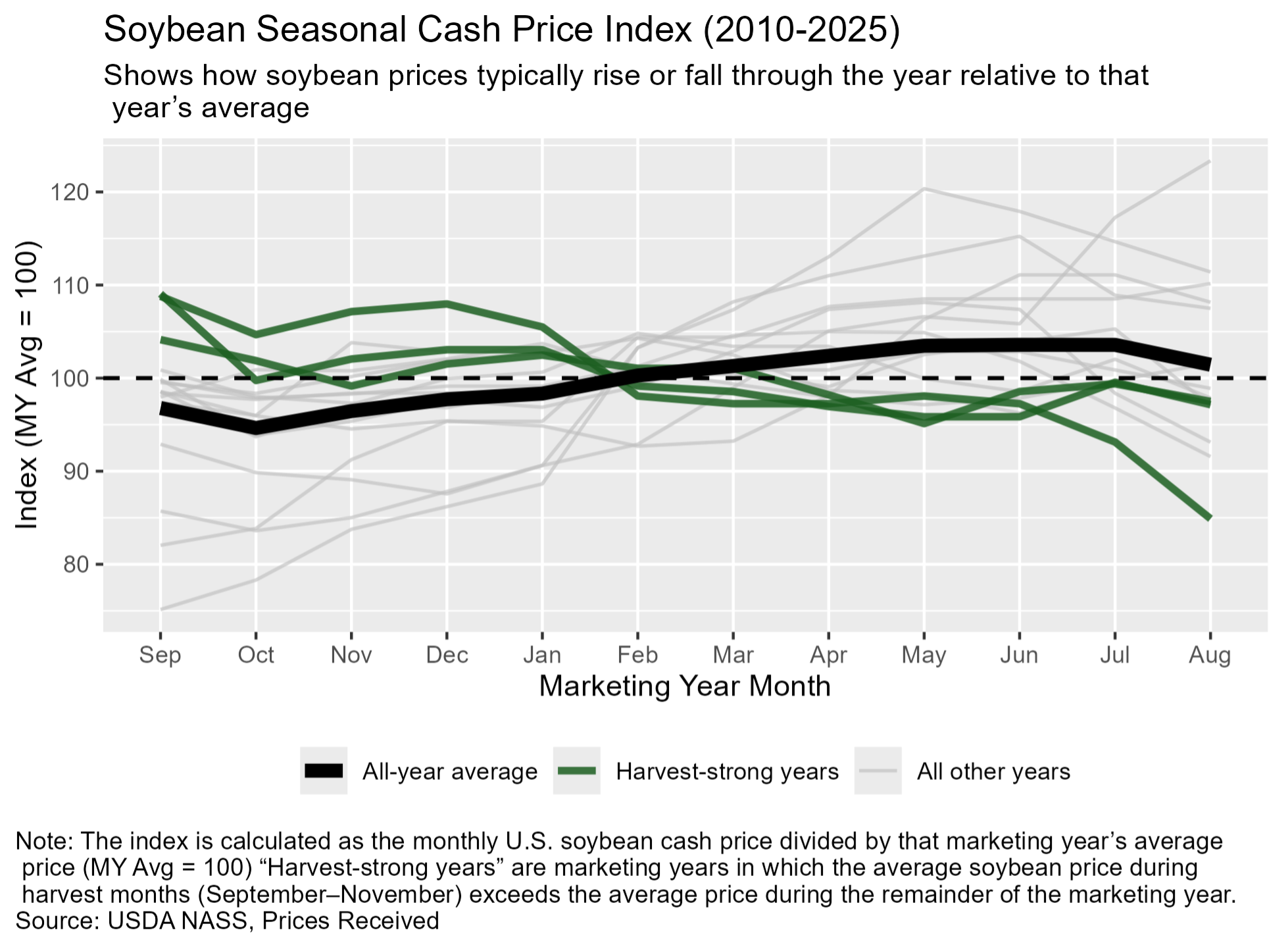
    Seasonality can help structure tiered price targets. As shown in Figure 1, the 10 year average soybean futures price, using the November contract pre-harvest and a nearby series post-harvest, tends to rise through the growing season as weather uncertainty builds, soften ahead of harvest pressure, and often strengthen again after harvest as stored supplies are rationed. While this pattern is not guaranteed in any given year, it provides useful context for historically favorable pricing windows. Producers might consider setting an initial pre-harvest target in the spring or early summer when weather-driven volatility supports prices, with additional tiers near typical post-harvest seasonal highs. However, post-harvest targets must account for carrying costs, including storage, interest, shrink, and quality risk, since higher futures prices do not necessarily translate into higher net returns if those costs outweigh the seasonal gain.

    Ultimately, a good price is influenced by farm-specific factors unique to each operation. By grounding price targets in cost of production, financial goals, basis expectations, and seasonal tendencies, producers can move from asking “Is this a good price?” to confidently knowing when a price meets their operation’s needs.

    Figure 1. Ten-Year Average Soybean Futures Prices Across the Pre- and Post-Harvest Marketing Window

    Note: Pre-harvest prices reflect the November soybean futures contract. Post-harvest prices are based on a continuous nearby futures series.

    Maples, William. “What Determines a “Good” Price?Southern Ag Today 6(10.3). March 4, 2026. Permalink

  • Global Stocks Are Up, Exporters Are Cutting Back, and U.S. Cotton Faces a Tough 2026

    Global Stocks Are Up, Exporters Are Cutting Back, and U.S. Cotton Faces a Tough 2026

    Authors: Yuri Calil and John Robinson

    Cotton prices remain low and moving sideways. Nearby futures and U.S. spot stayed weak into early 2026 (about $0.63/lb). New-crop Dec’26 futures still carry about a $0.06/lb premium over nearby futures, signaling the market expects some tightening later in the year. The carry in the futures market is not a reason to plant more cotton. It reflects the market pricing in an expected supply contraction, not a demand-led recovery.

    The global balance sheet explains why prices are stuck. For 2025/26, USDA projects 119.9 million bales of production and 118.7 million bales of mill use, raising ending stocks to 75.1 million bales. The U.S. picture is equally heavy: ending stocks reach 4.4 million bales, pushing the domestic stocks-to-use ratio to 32%, matching the highest level since the 2019/20 pandemic-era peak of 43%, with the season-average upland price lowered to $0.60/lb (USDA, 2026). High stocks slow any recovery unless demand surprises higher, which has not happened. This shifts attention to where supply cuts may emerge.

    Exporter production signals are mixed, but the direction is clear (Figure 1). The United States projects 13.9 million bales in 2025/26, down 3.5%, with flat harvested area (7.80 million acres) and a yield-driven decline. Australia shows a sharper pullback: production drops 19.6% to 4.5 million bales, driven by a 21.7% area cut as the Murray–Darling Basin enters a second dry season. Brazil is the swing case where the USDA projects 18.75 million bales (+10.3%), while CONAB is lower at 17.47 million bales with area down 3.1% and a lower yield. Those differences matter because Brazil can set the marginal export tone.

    Trade is where price pressure shows up first. USDA puts 2025/26 world trade up slightly at 43.7 million bales. Within that total, origins are shifting (Figure 2). The U.S. is gaining ground in Vietnam, while trade developments increase sales prospects to Bangladesh and India. But China appears to lean more toward Australia; February updates cut U.S. exports by 200,000 bales while raising Australia’s by 200,000 bales (USDA, 2026). When buyers switch origins, basis, and export bids can move fast.

    Acreage does not look like a bullish lever. The National Cotton Council projects 9.0 million cotton acres for 2026, down 3.2% from 2025 (NCC, 2026). Relative prices still favor competing crops, with the Dec’26 corn-to-cotton ratio near 6.7 points,[1] indicating flat-to-lower cotton acres, not expansion. Weather is the swing factor. NOAA expects La Niña to fade toward ENSO-neutral in Feb–Apr 2026 (60% chance), but parts of Texas entered late winter with drying soils and expanding drought, which can raise abandonment risk (NOAA CPC, 2026; USDM/NIDIS, 2026). If spring rains miss, supply could tighten into the new crop, consistent with the Dec’26 premium in futures.

    For U.S. growers, the playbook stays defensive, but flexible. Growers may wish to consider using rallies to price a portion of expected production and protect downside risk. Brazil’s acreage follow-through should be monitored, as well as China’s import pace, because both variables can change export competition quickly. Marketing should be tied to your cost structure and moisture outlook, since yield risk can dominate net revenue.

    Figure 1. Area vs. Yield: What’s Driving Exporter Production Shifts (2024/25 vs. 2025/26)

    Sources: USDA WASDE (February 2026), CONAB (February 2026). ABARES (December 2026). All data have been converted to acres, lbs/acre, and bales. Rectangles compare cotton production across the United States, Brazil, and Australia. Rectangle height is harvested area and width is yield, so rectangle area is proportional to production; dashed outlines show 2024/25 and solid rectangles show 2025/26.
     

    Figure 2. Cotton Trade: Major Exporters and Key Buyer Markets (2025/26)

    Source: USDA FAS (2026). Each ribbon represents a cotton export flow from an origin country (left) to a destination country (right). Ribbon width is proportional to volume in million 480-lb bales. 


    [1] The December corn-to-cotton price ratio is calculated as the December Corn futures price (CBOT ZCZ26, $/bu) divided by the December Cotton No. 2 futures price (ICE CTZ26, ¢/lb). Because the contracts use different units, this ratio is a rule-of-thumb indicator of relative new-crop price incentives rather than a direct profitability comparison. It is best interpreted alongside expected yields, local basis, and per-acre variable costs when assessing acreage shifts.


    References

    Australian Bureau of Agricultural and Resource Economics and Sciences (ABARES). (2025, December). Agricultural commodities: December quarter 2025 (Report No. 216). https://www.agriculture.gov.au/abares/research-topics/agricultural-outlook/australian-crop-report

    Companhia Nacional de Abastecimento (CONAB). (2026, February). Acompanhamento da safra brasileira de grãos: 5º levantamento, safra 2025/26. https://www.conab.gov.br/info-agro/safras/graos/boletim-da-safra-de-graos

    National Cotton Council of America (NCC). (2026, February). 45th annual early season planting intentions survey. https://www.cotton.org/econ/cropinfo/cropdata/planting-intentions.cfm

    National Integrated Drought Information System (NIDIS). (2026, January 22). Drought status update: Southern Plains. NOAA. https://www.drought.gov/drought-status-updates/drought-status-update-southern-plains-2026-01-22

    NOAA Climate Prediction Center (NOAA CPC). (2026, February 12). ENSO diagnostic discussion. National Weather Service/NCEP. https://www.cpc.ncep.noaa.gov/products/analysis_monitoring/enso_advisory/ensodisc.shtml

    U.S. Department of Agriculture, Agricultural Marketing Service (USDA AMS). (2026, February). Cotton market news — daily settlement prices. https://www.ams.usda.gov/market-news/cotton

    U.S. Department of Agriculture, Foreign Agricultural Service (USDA FAS). (2026, February). Cotton: World markets and trade. https://fas.usda.gov/data/cotton-world-markets-and-trade

    U.S. Department of Agriculture, World Agricultural Outlook Board (USDA WAOB). (2026, February 10). World agricultural supply and demand estimates (WASDE-668). https://www.usda.gov/oce/commodity/wasde/wasde0226.pdf


    Cali, Yuri, and John Robinson. “Global Stocks Are Up, Exporters Are Cutting Back, and U.S. Cotton Faces a Tough 2026.” Southern Ag Today 6(9.3). February 25, 2026. Permalink

  • 2026 Rice Market Outlook

    2026 Rice Market Outlook

    Authors

    Ryan Loy, Assistant Professor, University of Arkansas

    Alvaro Durand-Morat, Associate Professor, University of Arkansas

    2025 Domestic Market Recap and 2026 Outlook

    In 2025, U.S. rice acreage amounted to roughly 2.8 million acres, of which 2.7 million acres were harvested (USDA-NASS, 2026). All rice class acreage was down about 4 percent from 2024, due in part to the generational flood event that took place in April across the Midsouth, which forced many farmers to replant, or in some cases leave ground fallow due to razor-thin margins for rice in the South (Biram et al., 2025).  Compared to 2025, the upcoming growing season preview shows tighter stocks, with a declining price environment. The January 2026 WASDE report currently pegs long grain ending stocks at about 34.6 million bushels, little changed from the 24/25 marketing year but with a significant change in average farm price, which is currently forecasted at $10.50/cwt (down from $14.00/cwt during the 24/25 marketing year) (USDA, 2026). 

    2026 International Trade Outlook 

    International rice prices remain low due to large exportable surpluses, particularly from Asian exporters, and lower import demand from Indonesia. Temporary price increases, such as those observed in Thailand in late 2025, have already reversed, and export prices across major suppliers—including the United States, Uruguay, Thailand, and Vietnam—show sharp year-on-year declines (FAO, 2026). Unless major production shocks occur in Asia, prices are expected to remain depressed through 2026.

    Global rice production for the 2025/26 campaign is projected to be near record levels (around 541 million metric tons), with demand slightly lower (538.6 million metric tons), resulting in a third consecutive year of global surplus and continued stock accumulation (USDA-FAS, 2026). India has emerged as the world’s leading rice producer, surpassing China since 2024/25, and it is expected to reach a new production record in 2025/26 (preliminary reports suggest a record high main Kharif crop harvested in 2025 and an increase in area planted of the second Rabi crop). Its rapidly growing exportable surplus makes India a decisive force in shaping global market dynamics.

    Since U.S. long-grain rice competes strongly with Mercosur rice in the Western Hemisphere, it is important to highlight that the upcoming 2025/26 Mercosur harvest is expected to be smaller due to reduced planted area and climatic challenges, although high initial stocks—especially in Brazil—will partially offset lower output (USDA-FAS, 2026). Thus, Mercosur’s lower production performance may be good news for U.S. rice, maintaining or reclaiming market share throughout the Western Hemisphere. 

    In this international context, U.S. long-grain exports in the first half of marketing year 2025/26 (August-January) decreased 31% relative to the same period a year ago (Figure 1). While the U.S. has maintained export levels to Haiti and Iraq, it has experienced a significant drop in exports to Mexico and, to a lesser extent, to Canada and Honduras, due largely to increasing competition from South America.  

    Figure 1. U.S. long-grain exports during August-January of the marketing year – total and by top five destinations.

    References

    Biram, H.D., Loy, R., Hardke, J., Kelley, J., Ross, J., and Davis, J. 2025. Analysis Suggests Historic Flooding Results in $99 Million in Crop-Related Damages. University of Arkansas Factsheet. FSA93. Available online at, https://uaex.uada.edu/publications/PDF/FSA93.pdf.

    United States Department of Agriculture, National Agricultural Statistics Service. 2026. Crop Production: 2025 Summary. Available online at, https://esmis.nal.usda.gov/sites/default/release-files/795725/cropan26.pdf.

    United States Department of Agriculture. 2026. World Agricultural Supply and Demand Estimates. Available online at, https://www.usda.gov/oce/commodity/wasde/wasde0126.pdf.

    FAO Rice Price Update. Available online at https://www.fao.org/markets-and-trade/commodities/rice/fao-rice-price-update/en/  

    United States Department of Agriculture, Foreign Agricultural Service. 2026. Production, Supply and Distribution Online. Available at https://apps.fas.usda.gov/psdonline/app/index.html#/app/advQuery

    United States Department of Agriculture, Foreign Agricultural Service. 2026. Export Sales Reporting. Available at https://apps.fas.usda.gov/esrquery/esrq.aspx  


    Loy, Ryan, and Alvaro Durand-Morat. “2026 Rice Market Outlook.Southern Ag Today 6(8.3). February 18, 2026. Permalink

  • February WASDE Report Quiet while Soybean Futures Keep Moving Up

    February WASDE Report Quiet while Soybean Futures Keep Moving Up

    The USDA released the February World Agricultural Supply and Demand Estimates (WASDE) report yesterday with relatively little fanfare, especially compared to January.  Wheat showed a little lower domestic use, resulting in higher ending stocks.  Alternatively, corn showed greater exports and a lower ending stock, down to 2.1 billion bushels.  Both the wheat and corn price projections remained unchanged at $4.90 per bushel for wheat and $4.10 per bushel for corn.  The futures market for wheat and corn was essentially flat in response.

    The most active part of a quiet report day was with soybeans.  While domestic supply and use projections remained unchanged, production in Brazil was increased 2.0 million tons to 180.0 million tons.  This was as a result of both greater reporting area in Brazil and favorable weather conditions, contributing to an increase in global production and ending stocks.  However, the nearby futures market for soybeans maintained its upward trajectory, increasing roughly 11-12 cents per bushel, continuing the trend that started February 4 when soybean futures increased over 26 cents on comments by President Trump about China purchasing more soybeans.  Regarding China, the WASDE report indicated that, “China is reported to be considering buying more U.S. soybeans, … [but] if China bought more from the United States, global soybean exports will likely be shifted with more U.S. shipments to China and less to other markets.”  Thus, no change in global soybean demand was made in this report.

    Meanwhile, the balance sheet for cotton remained basically unchanged, with exports reduced 200,000 bales and the marketing year average price decreasing 1 cent to 60 cents per pound.  Table 1 details the current balance sheet for the four major crops.  Upcoming USDA activity to watch includes the release of the USDA Agricultural Baseline Projections to 2035, the 102nd Agricultural Outlook Forum, and then the March WASDE and Prospective Plantings reports.

    Table 1. 2025/26 Wheat, Corn, Soybean, and Cotton Supply, Use, Stocks, and Price Estimates, February 2026 WASDE

     WheatCornSoybeanCotton
     Production and Supply
    Planted (Million Acres)45.398.881.29.28
    Harvested (Million Acres)37.291.380.47.80
    Yield (Bushels/Pounds)53.3186.553.0856
    Production (Million Bushels/Bales)1,98517,0214,26213.92
    Total Supply (Million Bushels/Bales)2,95918,5974,60717.92
     US Exports and Use
    Exports (Million Bushels/Bales)9003,3001,57512.00
    Total Use (Million Bushels/Bales)2,02816,4704,25713.60
    Exports % of Total Use44%20%37%88%
     Stocks and Price
    U.S. Ending Stocks (Million Bushels/Bales)9312,1273504.4
    U.S. Stocks/Use46%13%8%32%
    U.S. Avg. Farm Price ($/Bushel or Pound)$4.90$4.10$10.20$0.60

    Data Source: USDA February 2026 WASDE


  • Price Seasonality: What the Pattern Shows

    Price Seasonality: What the Pattern Shows

    Commodity prices are influenced by a wide range of factors, but seasonal patterns remain an important consideration for crop marketing decisions. Even in periods of heightened volatility, understanding how prices tend to behave at different points in the marketing year can help producers evaluate timing risk and opportunity. Using soybeans as an example, this article examines historical price seasonality to illustrate how these recurring patterns can inform marketing strategies.

    Seasonality reflects the tendency for prices to follow recurring patterns throughout the marketing year, largely driven by changes in supply availability. Across crops, prices are often weakest near harvest, when supplies are most abundant, and strengthen later in the year as stocks are drawn down. While this pattern is widely understood, it is not universal. In some years, crop prices are stronger at harvest than during the remainder of the marketing year; however, these “harvest-strong” years are relatively rare and tend to behave differently than the typical seasonal pattern.

    Figure 1 illustrates soybean cash price seasonality using national monthly prices from 2010–2025. Prices are expressed as an index, calculated by dividing each month’s price by that marketing year’s average price. A value of 100 represents the average price for the year, while values above (below) 100 indicate prices that were higher (lower) than average.

    The thick black line in Figure 1 shows the average seasonal pattern across all years. This long-run average confirms a familiar story: soybean prices tend to be relatively weaker in the early fall, strengthen through winter and spring, and often peak in late spring or early summer before declining as new-crop supplies approach. From a seasonal perspective, this pattern suggests that pre-harvest and late-spring marketing opportunities often outperform harvest-time sales.

    Not all years follow this average path. The green lines in Figure 1 highlight harvest-strong years—marketing years in which average soybean prices during harvest (September–November) were higher than prices during the remainder of the marketing year. The lighter gray lines represent all other years. Over the past 15 years, soybean prices were higher at harvest in only three years: 2015, 2019, and 2024. In 2015, harvest prices were supported by weather risk and relatively tight global balance sheets. In 2019, prices were influenced by trade uncertainty and a delayed supply response. Most recently, in 2024, tight stocks and global supply concerns helped support prices at harvest. In contrast, the remaining years exhibit stronger pricing opportunities outside the harvest window.

    This distinction has practical marketing implications. In most years, weak harvest prices are followed by some degree of seasonal recovery, making post-harvest marketing opportunities more attractive. When prices are unusually strong at harvest, however, the historical record suggests that price upside later in the marketing year may be more limited.

    The key takeaway is not that producers should market at the same time every year, but that seasonality provides a useful baseline expectation. When prices align with typical seasonal patterns, historical averages can help frame marketing decisions. When prices deviate, particularly when harvest prices are strong, it may signal that capturing favorable prices sooner deserves consideration. Incorporating seasonal patterns alongside market fundamentals, risk tolerance, and cash-flow needs can help producers make more disciplined and informed soybean marketing decisions.

    Figure 1.


    Gardner, Grant. “Price Seasonality: What the Pattern Shows.Southern Ag Today 6(6.3). February 4, 2026. Permalink