The 2025 trade war between the U.S. and China has been an evolving phenomenon. The U.S. implemented tariffs on Chinese imports effective February 4, which were then increased March 4. China responded with a variety of tariffs, including 15% additional tariffs on U.S. raw cotton, effective March 10.
The above situation continued to change, with the U.S. and China effectively embargoing their mutual trade in April with extreme tariff levels and then adjusting these extreme levels lower in May. As of May 12, and for 90 days, the Chinese tariff rate on U.S. cotton is 10%.
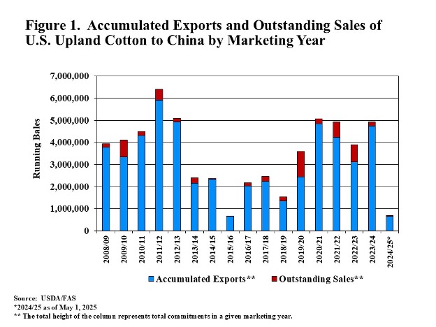
With all the policy variation, the direct impact on U.S. cotton has probably been lower in the current 24/25 marketing year than it would have been in previous years. The reason is that 2024/25 has seen an historically low level of U.S. export commitments to China of upland cotton (Figure 1). Thus, there is relatively little volume of U.S. cotton to be directly impacted by the initial, extreme, or current levels of Chinese tariffs.
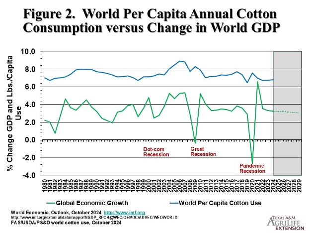
The remaining tariff risk to cotton demand is more likely an indirect influence. To the extent that tariffs imposed by the U.S. and its trading partners depress GDP, it follows that demand for semi-durable discretionary textile products could be reduced. This possibility is suggested in Figure 2, where the percentage change in world GDP appears to move directly with annual per capita cotton consumption.
The May 2025 World Agricultural Supply and Demand Estimates (WASDE) is a highly anticipated report as it offers the first official USDA estimates of the new crop marketing year (USDA, 2025). For 2025/2026, the estimates show a divergence of fundamental factors in the U.S. grain markets. Estimated days of use on hand at the end of the marketing year (a stocks-to-use ratio calculated by dividing ending stocks by average daily use) are projected to increase in 2025/2026 compared to 2024/2025 for corn, wheat, and rice. Conjointly, the season average farm price is projected lower for these three grains. For soybeans, days of use on hand are forecast to decrease and the farm price is forecast to increase compared to last year.
Based on the Prospective Plantings report back in March, corn acres for 2025 are projected at 95.3 million, up from 90.6 million in 2024. USDA’s yield estimate for 2025 is a record high 181.0 bushels per acre. This combines for a record corn crop of 15.820 billion bushels. Add in 1.415 billion bushels of beginning stocks and the corn supply in the 2025/2026 marketing year is a record 17.206 billion bushels, up 3.6% from last year.
U.S. corn use is projected at record levels as well with increases in feed and exports. However, the increase in corn supply exceeds the increase in use, resulting in an increase in ending stocks. Days on hand increased by an 8.6-day supply, and the season average farm price is down from $4.35/bu last year to $4.20/bu. With a PLC reference price in 2025 of $4.26/bu, that would earn a 6-cent-per-bushel payment.
Soybean acres for 2025 are estimated at 83.5 million, down from 87.1 million in 2024. But with a record forecast yield of 52.5 bushels per acre, production in 2025 is down only 26 million bushels from 2024. Soybean use is forecast to increase by 31 million bushels on increased domestic crushings. Ending stocks are expected to decrease by 55 million bushels, and days of use on hand are expected to decline by 4.8 days. The season average farm price is projected to increase by 30 cents per bushel to $10.25.
U.S. wheat production is estimated to be little changed from the 2024 crop with the decrease in acres mostly offset by a higher yield estimate. Impacting the wheat supply for 2025/2026 is an increase in beginning stocks and a decrease in projected imports (-30 million bushels). Wheat use is projected lower on a decrease in exports of 20 million bushels. This raises the wheat ending stock estimate by 82 million bushels, increases carryover to a 172-day supply, and lowers the season average farm price from $5.50/bu last year to $5.30/bu. With a $5.56/bu reference price, this would generate a PLC payment of 26 cents per bushel.
The U.S. rice supply in 2025/2026 is projected higher, as an increase in beginning stocks offsets a small decline in production. Use is up 1 million hundredweight with an increase in domestic use and a decrease in exports. This leaves ending stocks up 3.5 million hundredweight and days on hand higher by 3.2. The farm price is down $2 per hundredweight to $13.20, below the PLC reference price of $14.00.
Of course, much can change between these early season estimates and final crop production and use numbers. Weather, trade policies, the economy, global grain fundamentals, and other factors foreseen and unforeseen, will evolve and emerge to shape grain prices. The May WASDE is an important benchmark to assess and estimate the impact of these changes and forces as the season unfolds.
Table 1. May 2025 WASDE Numbers for U.S. Grains (corn, soybeans, and wheat in millions of bushels; rice million hundredweight) and 2025 PLC Reference Prices and Estimated Payment Rate.
Crop
Corn
Soybeans
Wheat
Rice
mil bu
change*
mil bu
change*
mil bu
change*
mil cwt
change*
Beginning Stocks
1,415
-348
350
+8
841
+145
45.0
+5.2
Production
15,820**
+953
4,340
-26
1,921
-50
219.3
-2.8
Total Supply
17,260**
+605
4,710
-24
2,882
+64
313.5**
+3.5
Total Use
15,460**
+220
4,415
+31
1,959
-18
266.0**
+1.0
Ending Stocks
1,800
+385
295
-55
923
+82
47.5
+2.5
Days on Hand
42.5
+8.6
24.4
-4.8
172.0
+16.7
65.2
+3.2
Price $/bu or $/cwt
Farm Price
$4.20
-$0.15
$10.25
$0.30
$5.30
-$0.20
$13.20
-$2.00
PLC Reference Price
$4.26
$9.26
$5.56
$14.00
PLC payment rate
$0.06
$0.00
$0.26
$0.80
*change 2025/26 marketing year compared 2024/25 marketing year.
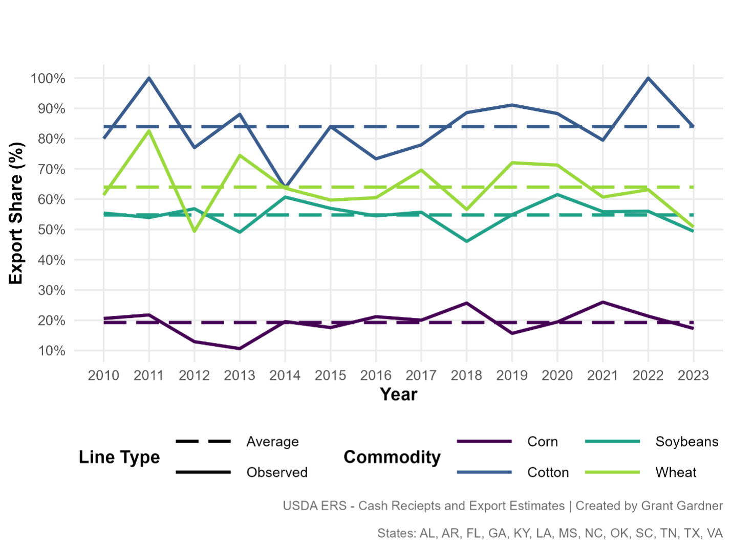
International markets support U.S. agriculture, especially in the Southern states. Exports make up a significant portion of cash receipts for many major commodities produced in the Southern states (Figure 1). From 2010 to 2023, an average of 84% of cotton receipts came from exports, underscoring the crop’s reliance on global trade. Wheat and soybeans also depend heavily on international markets, with exports accounting for 64% and 55% of their respective receipts. In contrast, corn is less export-oriented, with just 19% of receipts linked to foreign buyers[1]. This level of exposure makes Southern agriculture especially sensitive to tariff changes and trade policy shifts. During periods of uncertainty, a well-informed marketing and risk management strategy is often the best defense producers have against market volatility.
A well-developed marketing and risk management plan is essential for producers facing today’s volatile markets. While trade uncertainty is a significant source of price swings, volatility is a constant in agriculture—driven by weather, input costs, and global events. Trade is one of the dominant factors right now. Regardless of the cause, producers should expect uncertainty and be ready to manage price risk each crop year. A strong marketing and risk management plan is the best tool for navigating uncertainty. Crucially, the plan should be written down and shared with everyone involved in the operation to ensure clear communication and timely decisions. Growing a crop and marketing a crop involve two completely different skill sets, so communication between those in charge of production and those in charge of marketing and risk management is essential.
The most significant value of a marketing plan is determining sales timing, which should coincide with when production risk is reduced, and what action should be taken at different price points. Trying to time price peaks in markets shaped by unpredictable trade shifts is often ineffective and can be risky. Instead, a solid marketing plan sets decision dates, creating structure around when and how much to sell if markets achieve price targets. Dates should be tied to when production risk is reduced and be informed by realistic price targets, helping producers stay disciplined and focused on financial goals while taking some of the emotion out of pricing decisions. The key is to make sales when prices meet or exceed profit objectives at strategic points in the production/marketing year—even if prices might rise later. Especially in tight-margin years, locking in profits when available can be critical to the operation’s financial success.
Producers may benefit from a more proactive sales strategy in today’s challenging market environment when profit opportunities arise. For instance, a summer weather rally that pushes prices higher could present a good time to forward contract or price additional bushels before harvest. While aggressiveness in pre-harvest marketing will vary depending on each producer’s risk tolerance, defining that comfort level in advance is essential. The best marketing decisions are those made with forethought—not in the heat of the moment. In years with tight margins, relying on chance is a risk most operations can’t afford.
Figure 1. Export Contribution to Southern Ag Receipts, Observed and Average Share by Commodity, 2010-2023
[1] Estimates do not include by products for crops such as ethanol, dried distiller grains (DDGs), soybean oil, and soybean meal.
Farmers decide what crops to plant based on factors like crop rotations, expected profits, input costs, and other financial trade-offs. Annual predictions of planted acreage for a crop help agribusiness suppliers plan for seed, fertilizers, pesticides, and equipment needs. Prices of crops and how they compare to competing crops, like corn and cotton, influence planting decisions. In many southern states, corn competes with cotton for land, and the cotton-to-corn price ratio is a key factor in predicting how much land will be dedicated to cotton. Additionally, past planting decisions impact future choices due to crop rotation, which helps manage pests, diseases, and soil health while enhancing yield potential.
To estimate how much cotton farmers will plant in 2025, we built a model that looks at past cotton and corn prices, along with historical cotton acreage data. Data was obtained from the U.S. Department of Agriculture (USDA) National Agricultural Statistics Service (NASS) for 1990 to 2024. One of the most important factors in our model is the cotton-to-corn price ratio, which is calculated by dividing the cotton price (in cents per pound) by the corn price (in dollars per bushel).
By analyzing historical patterns, our model estimates how much cotton (total upland and Pima cotton acreage) will be planted next year based on three main factors: (1) last year’s cotton acreage; (2) the cotton-to-corn price ratio from the previous year; and (3) the expected cotton price for the upcoming year.
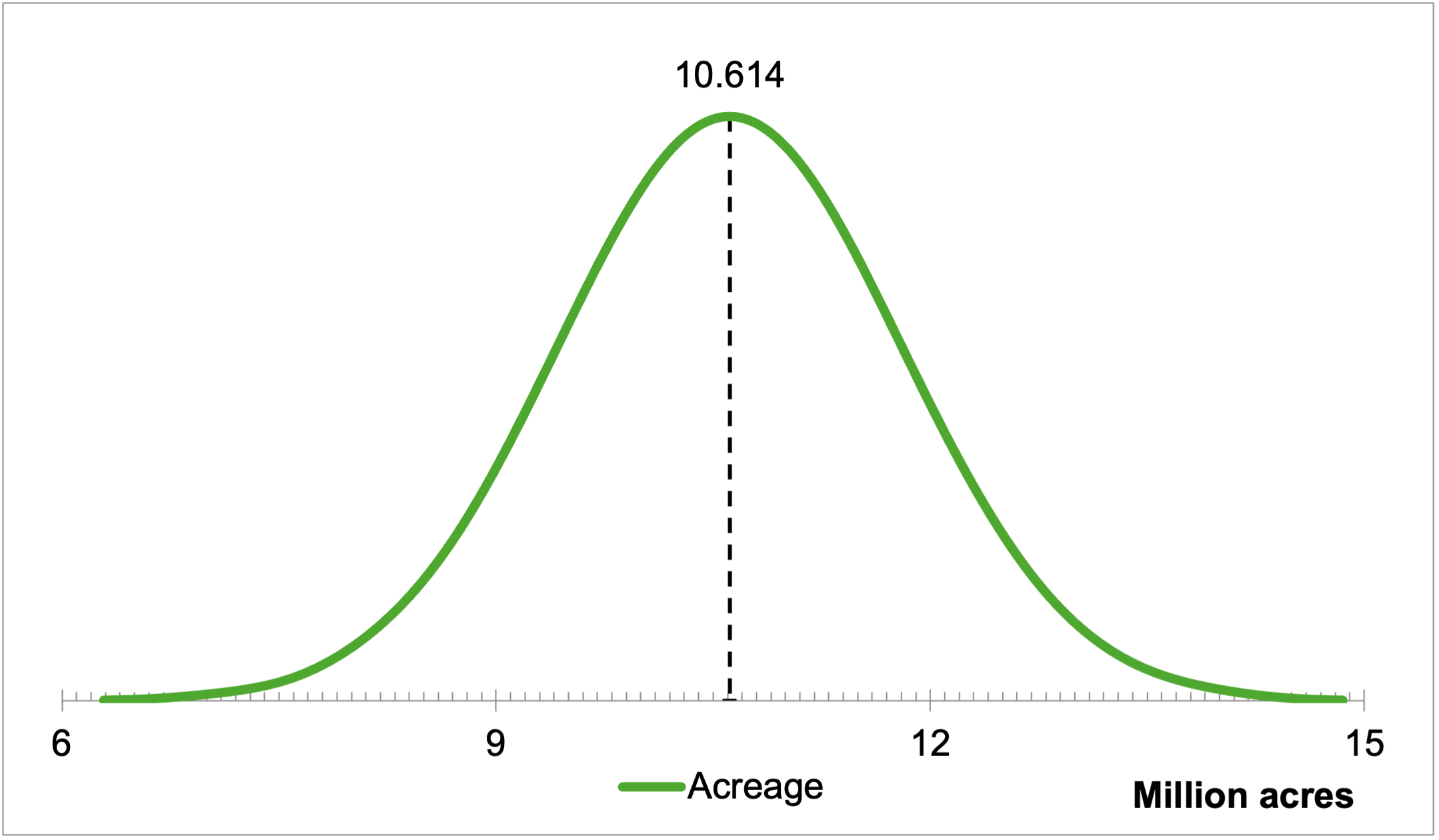
Simulated Cotton Planted Acreage in 2025
Using recent estimates from the USDA, we applied our model with a cotton-to-corn price ratio of 14.48 (based on a cotton price of 63.0 cents per pound and corn prices of $4.35 per bushel) as currently estimated by the April 2025 WASDE Report for the 2024 crops. A cotton price of 67.60 cents per pound for the 2025 crop is projected based on the February 2025 reported cotton price by USDA NASS.
Our model predicts that farmers will plant approximately 10.524 million acres of cotton in 2025 (Figure 1), a 5.88% decrease from 2024 (when 11.182 million acres of upland and Pima cotton were planted in total). This is higher than the 9.87 million acres forecast by the USDA Prospective Plantings report published on March 31, 2025. These projections, while containing a degree of uncertainty, help farmers and agribusinesses prepare for the upcoming season by anticipating cotton plantings and allowing adjustments in strategies accordingly.
Figure 1: Projected Probability of Total Upland Cotton and Pima Cotton Planted Acreage for 2025. Higher Points Indicate More Likely Acreage Outcomes for 2025 Based on Simulation Results.
The Ordinary Least Squares (OLS) regression results (Table 1) show that the previous year’s cotton acreage, the previous year’s cotton-to-corn price ratio, and the current year’s cotton price significantly impact current-year planting.
Table 1: Impact of Historical Cotton Acreage and Cotton-to-Corn Price Ratio on Future Cotton Planting Decisions
Independent variable
Coefficient
t-ratio
0.404*
3.491
256.451*
5.812
31.223***
1.828
272.209
0.117
F-test
22.092
0.688
34
*, **, *** indicates significance at the 99%, 95% and 90%, respectively.
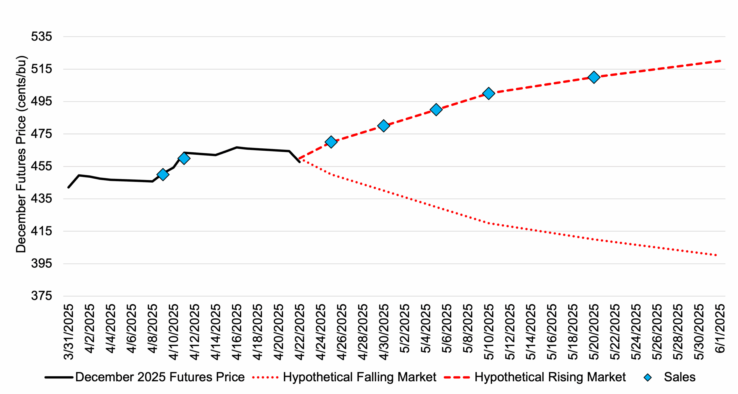
Tariff escalation remains a major source of uncertainty that could substantially move corn futures markets in the coming weeks/months. Managing some futures price risk based on the current rally is worth considering given the uncertainty in corn markets. On Friday April 11, December corn futures broke through a key resistance point at $4.60/bu. For those farmers that have not started pricing the 2025 crop, December corn futures above $4.50/bu represent a good starting point to remove some futures price risk (basis could be secured now or left to be fixed at an alternative date depending on local basis offerings). Pricing into a futures market rally, through incremental sales, is a strategy worth considering, and one that will take some of the emotion out of marketing decisions. For example, starting at a December futures price of $4.50/bu, consider pricing 5% of projected 2025 production. For each additional 10-cent increase in futures price, consider establishing a futures price on an additional 5% of estimated production up to a maximum of 35% of projected 2025 production. Pricing more than 35% of the crop before June can be risky and can result in exchanging price risk for production risk or having limited production to price should a bullish weather market occur in June/July/August. The maximum amount to be priced before June can be a personal preference based on the farmers’ risk tolerance, variability in yield for the farm, and access to storage. This incremental pricing strategy would establish an average futures price of $4.80/bu on 35% of projected production if the December corn futures price rallied to $5.10/bu (Figure 1). However, it would also put some sales (10% of estimated production at an average price of $4.55/bu as of April 22) on the books if the current rally stalled or reversed. Futures prices above $4.50 plus a positive basis, which occurs in most Southern states, will result in cash prices of nearly $5.00.
Table 1. December Corn Futures Price and Sales into a Hypothetical Rising or Falling Market