The Poultry Grower Payment Systems and Capital Improvement Systems rule proposal is the latest effort by the Agricultural Marketing Service to address perceived inequities within the typical commercial broiler grower’s contract arrangements with poultry companies like Tyson, Pilgrims, and others. This is in addition to the recently passed Transparency in Poultry Grower Contracting and Tournaments rule, which became active on February 12, 2024. The proposed new rule would also modify the Packers and Stockyard Act. If implemented, the new rule would affect poultry growers in two substantial ways: 1. It would change the primary way most contract broiler growers are paid by modifying or replacing the traditional “tournament pay ranking system” (only applies to companies using such a ranking system) and 2. it would establish documentation requirements for any additional capital improvements recommended or required by the company. The comment period for this rule closed on August 9, 2024. The final results of this proposed rule may be impacted by the recent SCOTUS decision in Loper Bright on federal agencies’ rulemaking power to implement such rulings.
The traditional tournament pay system allows for the grower’s pay per pound to be adjusted up or down, or “ranked”, from a stated base pay rate according to the cost of growing the company’s birds on individual contract farms. Broiler growers are typically subject to “pluses and minuses” above or below a stated base pay per pound. (see fig 1) This ranked pay system has been in place for most contract growers in some form for several decades. The most often noted concern is that it can cause growers to receive a lower pay rate based on factors not fully in their control. Many companies recognize this potential and have contingency plans that offer growers relief from such situations, though not all agree on how those are handled or when they are appropriate. From a practical perspective, sometimes the exact cause of a high-cost flock of chickens is difficult to identify. Even so, growers often feel they are at the mercy of a system not designed with their best interests in mind. The proposed rule would attempt to remedy this situation by requiring all contracted growers to receive a minimum pay rate for every flock, regardless of a flock’s cost to the company. The rule does not specify whether this pay must be per pound, per square foot of growing space, or any other specific method. It does specify that any pay system must be a “fair comparison among growers.” The rule would allow positive pay incentives to be utilized, but only if all stipulations for receiving incentives meet the “fair comparison among growers” standard and are clearly documented.
Simply put, under the new rule, there could be competition for extra pay, but everyone gets the minimum pay first. Any grower who experiences a non-competitive situation out of their control would be required to be paid outside of any competition. It is suggested that a multiple flock average payment be employed in such cases. (Many poultry companies use a multi-flock average in such situations now.) The rule also stipulates that the minimum pay cannot be set arbitrarily low but must be sufficient to cover the average costs of growing birds in an area.
Whether or not a new pay system would increase the cost of growing birds for a company would depend on the system and rates chosen. However, if there is a minimum pay guarantee, it is plausible that minimum standards for raising the birds will be increased. It is also plausible that the highest pay rates a grower could earn might be decreased to cover company live-cost increases from a new system of pay.
The second part of the rule concerns capital assets on the farm. Often, companies recommend or require growers to make significant capital investments in equipment upgrades or structural improvements. Sometimes, these are simply “good maintenance” related, but often, they concern efficiency or cost-saving improvements that benefit the company as much as the grower. They could be the result of customer’s demands or animal welfare guidelines. Under the new rule, companies that recommend or require additional capital improvements of $12,000 or more must provide documentation to the grower of why such expenditures are to be made, expected costs, potential benefits to the grower or the birds, the research or data that supports it, and what the grower should expect for financial return, if any. The rule does not eliminate the potential of a grower suffering a negative impact if a specific required capital improvement is not implemented. Nor does it require that all capital expenditures be financially beneficial to growers. It simply requires the documentation above with some financial explanation for any additional capital improvement coming from the company.
In addressing the overall purpose of this proposed rule, the following statement was made in summary by the AMS:
“The benefits that will accrue to growers from the proposed changes will result from increased clarity as growers will be informed of minimum compensation outcomes that can occur under the broiler grower arrangement. There is no expectation that aggregate payments to growers will increase.”
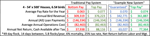
Fig. 1: In a traditional tournament pay system, there could be a range of +/- 10% or more from base pay per pound delivered. A grower’s pay could vary anywhere in this range based on their flock’s cost. This doesn’t sound like much variation, but when multiplied over the total pounds of a modern farm, the resulting gross revenue differential is substantial. In the examples below, if base pay is $0.070 / lb., top pay is $0.077 and bottom pay is $0.063 per pound under a traditional tournament system, the resulting pay variation a grower might experience flock to flock could be $8,650, or $50,178 total annually. Under the proposed rule, the base pay would now be the minimum per pound guaranteed to the grower. It is plausible that the resulting top pay might be lowered to +5% to help the company cover the potential increase in live-cost, resulting in lower potential top pay for growers. However, the potential variation might decrease to $14,337 annually under a “new” system, lessening the income risk of the grower by 60%.
Brothers, Dennis, and Paul Goeringer. “Contract Broilers Growers Could See Changes in Their Pay Arrangements.” Southern Ag Today 4(39.1). September 23, 2024. Permalink