Authors: Susmitha Kalli, Graduate Student, Department of Agricultural and Applied Economics, University of Georgia; Yangxuan Liu, Associate Professor, Department of Agricultural and Applied Economics, University of Georgia; Hunter D. Biram, Assistant Professor, Department of Agricultural Economics and Agribusiness, University of Arkansas; Fayu Chong, Graduate Student, Department of Forest Resources and Environmental Conservation, Virginia Tech University
Federal crop insurance remains a vital risk management tool for peanut producers across the United States. In our previous Southern Ag Today article, we discussed the various crop insurance policies available for peanuts. As with other crops, securing and maintaining insurance coverage for peanuts requires close attention to key administrative deadlines set by the U.S. Department of Agriculture’s Risk Management Agency (USDA RMA). Two of the most important are the sales closing date and the cancellation date, which determine eligibility and the continuation of coverage for each crop year.
The sales closing date is the final day producers can apply for insurance or make changes to an existing policy. This includes selecting the type and coverage level. The cancellation date is the deadline for producers to notify their insurance provider in writing if they choose not to renew their policy. Policies not canceled by this date are automatically renewed under existing terms. For peanuts, the sales closing date and the cancellation date are the same for a given location and are uniform across all available crop insurance policies.
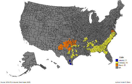
While these dates remain consistent year to year, their timing varies by state and county. Notably, USDA RMA divides Texas into three distinct regions, each with different deadline dates, whereas other peanut-producing states follow a uniform date statewide, as shown in Table 1 and Figure 1.
These deadlines are especially important for producers who contract with a sheller. Although insurance coverage is available for all insurable peanut acreage, regardless of whether the crop is grown under contract, the valuation of indemnities may differ depending on contract status. Specifically:
- Contracted peanuts: When the crop is grown under a qualifying sheller contract, the contract’s base price may be used to calculate coverage, subject to USDA RMA guidelines.
- Non-contracted peanuts: When the crop is not contracted, indemnities are based on a price election determined by USDA RMA.
- Mixed production: For producers growing both contracted and non-contracted peanuts, coverage can be divided accordingly, provided that all sheller contracts are submitted by the acreage reporting date.
To avoid missing critical deadlines or encountering coverage limitations, producers are strongly encouraged to verify their county-specific requirements using the USDA RMA Actuarial Information Browser. A certified crop insurance agent can also assist in clarifying enrollment options, contract documentation requirements, and eligibility based on production practices. The USDA RMA Agent Locator Tool provides a searchable database that helps producers connect with authorized crop insurance representatives in their state.
Table 1. Peanut Crop Insurance Policies’ Sales Closing Dates and Cancellation Dates by State and County
| Region | States and Counties Covered | Dates |
| South Texas Counties | Includes Jackson, Victoria, Goliad, Bee, Live Oak, McMullen, La Salle, Dimmit, and all Texas counties lying south of this line | Jan 31 |
| Central/Eastern Texas and Most Other States | Covers Alabama, Arkansas, Florida, Georgia, Louisiana, Mississippi, North Carolina, South Carolina, and parts of Texas including El Paso, Hudspeth, Culberson, Reeves, Loving, Winkler, Ector, Upton, Reagan, Sterling, Coke, Tom Green, Concho, McCulloch, San Saba, Mills, Hamilton, Bosque, Johnson, Tarrant, Wise, and Cooke, as well as all Texas counties lying south and east of this boundary | Feb 28 |
| Remaining Areas | Includes all other Texas counties not listed above, along with New Mexico, Oklahoma, and Virginia | Mar 15 |
Figure 1. Regional Differences in Sales Closing Dates and Cancelation and Termination Dates Runner-Type Peanut Crop Insurance*
References
USDA Risk Management Agency (USDA RMA). Peanut Crop Provisions 20-PT-075. Available at: https://www.rma.usda.gov/policy-procedure/crop-policies/peanut-crop-provisions-20-pt-075
USDA Risk Management Agency. Actuarial Information Browser. Accessed April 2025. https://webapp.rma.usda.gov/apps/ActuarialInformationBrowser/
USDA Risk Management Agency. Agent Locator Tool. Accessed April 2025. https://public-rma.fpac.usda.gov/apps/AgentLocator/#!/
Kalli, Susmitha, Yangxuan Liu, Hunter D. Biram, Fayu Chong. “Peanut Crop Insurance: Differences in Sales Closing Dates and Cancellation Dates Across Regions.” Southern Ag Today 5(50.1). December 8, 2025. Permalink