Pasture, Rangeland, and Forage (PRF) insurance has become a key risk management tool for ranchers and forage producers looking to protect themselves against the unpredictability of rainfall. However, like all insurance products, PRF comes with its own set of risks. In this article, we explore the risk associated with producer interval selection and its potential downsides and upsides.
A unique risk with PRF insurance is that rainfall during a particular two-month interval does not necessarily lead to forage growth during that interval. Rainfall is obviously crucial for forage production, but the impact of precipitation on forage is not instantaneous. Often, rain that occurs during one interval may contribute to forage growth in the following months more than the month in which the rain occurred. Therefore, choosing a PRF interval that aligns directly with your critical forage production interval could potentially be a mismatch.
A downside of this timing mismatch is that a producer may not receive an indemnity payment when needed. For instance, if the insured interval experiences average rainfall but the interval prior had low precipitation or the rain came towards the end of an interval, the forage growth may still be insufficient. Unfortunately, since the payment is based strictly on the rainfall during the insured interval, producers might not receive any payout despite facing significant challenges. The chance of this outcome occurring is considered a False Negative Probability (FNP). False in the sense that the signal (rainfall) did not correspond with the underlying production need (forage production), and negative in that the outcome provided no protection when you needed it.
On the flip side, this same mismatch can work in favor of producers. Suppose the insured interval experiences low rainfall, but the previous interval had good precipitation. In that case, sufficient forage growth can occur in the insured interval, and the insured can still receive an indemnity payment. The likelihood of the PRF policy providing a payment even when forage conditions are favorable is the False Positive Probability (FPP).
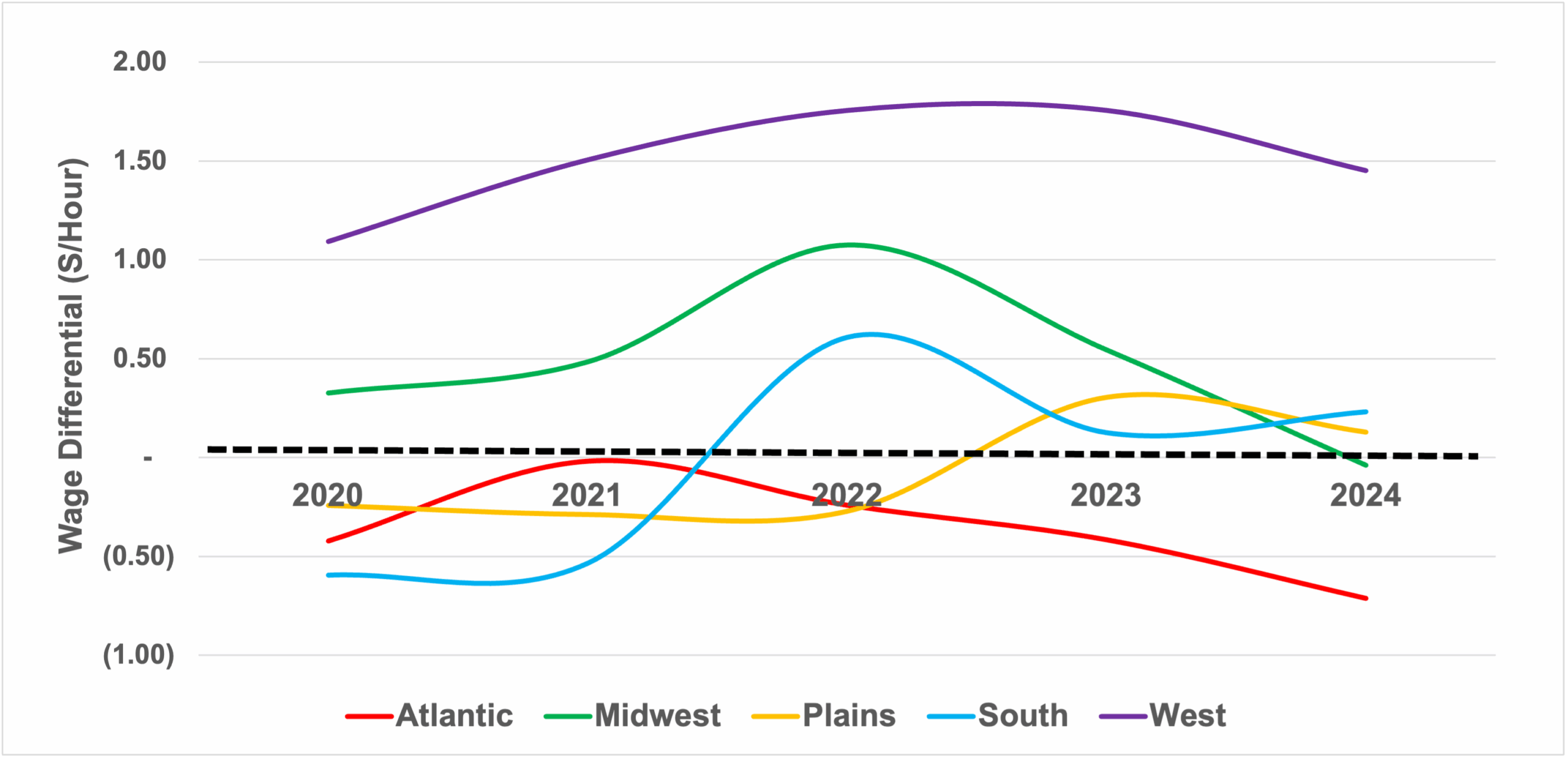
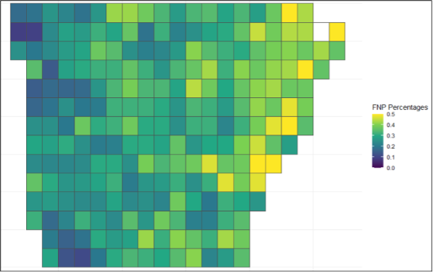
Figure 1 below illustrates this potential downside risk through the prevalence of FNPs in grids in Arkansas. These values were calculated by creating a forage/vegetation index to match the Rainfall Index used by the PRF program. Using Normalized Difference Vegetation Index (NDVI) values, we found the FNP percentages for each grid and each interval. Figure 1 highlights the June-July interval, telling us the percent chance that the forage/vegetation index would indicate a need for an indemnity based on the coverage level when the policy using the rainfall index has not been triggered (Keller & Saitone, 2022). This shows the prevalence of this issue and that producers in certain regions should be more wary of this type of risk.
A unique risk with PRF insurance is tha
Figure 1: False Negative Probability Percentages in Arkansas Grids for the June-July Interval (1981-2023)
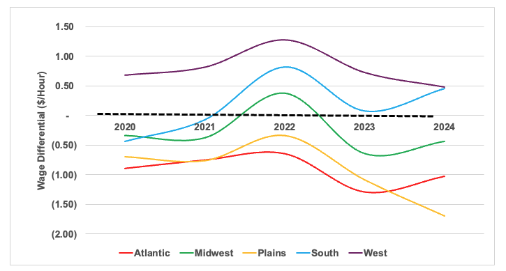
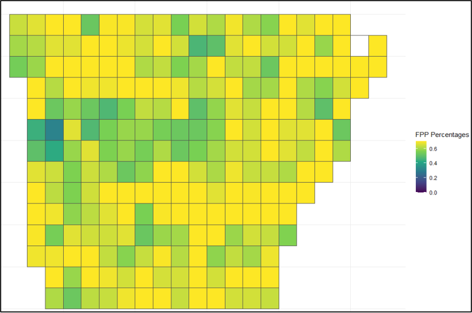
Inversely, Figure 2 presents the frequency of FPPs showing the upside risk. Reversing the methodology, these were calculated as the percent chance that the rainfall index indicates an indemnity should be issued based on the coverage level when the forage/vegetation index says an indemnity should not be issued. This scenario tends to be more prevalent, which is good for the policyholder. Certain grids exhibiting high FPPs also tend to show high FNPs, indicating they might frequently receive unwarranted payments while simultaneously facing situations where they do not receive payments when needed. This raises an issue with the producer, causing them to change how they manage their finances to protect themselves instead of the program doing so properly.
Figure 2: False Positive Probability Percentages in Arkansas Grids for the June-July Interval (1981-2023)
While these figures only highlight the prevalence of FNP and FPP in Arkansas, these risks are inherent in PRF and are just as likely in the other southern states. To counter this risk, producers should consider not only the months when forage is most needed, but also the months when moisture and precipitation are most important. Using this information, they can choose their PRF intervals appropriately and reduce the risks involved in the program.
References
Keller, James B., and Tina L. Saitone. 2022. “Basis Risk in the Pasture, Rangeland, and Forage Insurance Program: Evidence from California.” American Journal of Agricultural Economics 104 (4): 1203–23.
Davis, Walker B., Lawson Connor, and Hunter Biram. “Analyzing the Upside and Downside Risk in PRF Policy Selection: Timing Mismatch.” Southern Ag Today 5(21.1). May 19, 2025. Permalink