Agricultural economists receive requests for a variety of data from our clientele. One common question we receive during this time of year is about the going rate on cash land rents. The U. S. Department of Agriculture National Agricultural Statistics Service (USDA NASS) conducts an annual survey on cash land rental rates and publishes the results on its website by early August of each year.
Producers often rent a portion of the total land they farm. Part of this is because acquiring land is difficult due to scarcity, and the other part is because it takes significant capital to buy land. Farming on more acres by renting enables producers to more efficiently utilize their assets and achieve economies of scale through increased production while spreading their costs across more acres.
Producers can rent either irrigated or non-irrigated cropland. If the landowner has an established irrigation system in place, the rent on irrigated land is higher than the rent on non-irrigated land. In some instances, a producer can place temporary irrigation on the land they are renting. Since the producer owns and pays for the irrigation system, the rent expense is usually comparable to that of non-irrigated land. A variety of agreements can be made between the landowner and producer to accommodate their needs.
The following 2 figures show indices of average annual cash rents for the five years before and after the COVID-19 pandemic for irrigated (Figure 1) and non-irrigated (Figure 2) cropland. Land rents can vary significantly from parcel to parcel and state to state. An index was chosen instead of the actual value of cash rents per acre to allow for relative comparison between states. The year 2019 was chosen as the base year of the index because the rent values, published in August 2019, were not impacted by the pandemic. The scale of the y-axis on the irrigated and non-irrigated charts are the same with an index range from 70 to 140, although there is a much narrower range in observed non-irrigated land rents over the 11-year period from 2014 through 2024 than the observed range on irrigated.
Figure 1 shows a larger increase in average annual cash land rents on irrigated cropland during the 5-year period following the pandemic compared to the 5-years prior. South Carolina, Oklahoma, and Virginia saw a peak in average annual irrigated cash land rents in 2022, while North Carolina and Florida saw peaks in 2023. In 2024, these five states saw land rents come down slightly or stay about the same as their peak rates. The other states (Texas, Arkansas, Mississippi, Georgia, Alabama, and Louisiana) have seen rental rates continue to increase through 2024. Only Kentucky saw land rents below the 2019 average annual rate, except during 2023, when it was the same.
Figure 2 also shows a larger increase in average annual cash land rents on non-irrigated cropland during the 5-year period following the pandemic. However, the rate of increase is smaller than that of irrigated cropland. Alabama, Georgia, Kentucky, Louisiana, Mississippi, North Carolina, Oklahoma, Tennessee, and Texas saw their highest average annual cash land rents on non-irrigated cropland in 2024. South Carolina and Virginia saw a peak in 2023 and a slight decline in 2024. Florida saw a peak in 2020, with rents on non-irrigated cropland below the rate in 2019 for the other years after the pandemic. The only state to see land rents on non-irrigated cropland peak prior to the pandemic was Arkansas in 2015.
Figure 1. Index of Average Annual Cash Rents, Irrigated Cropland in the Southeastern U.S. (2019 = 100).
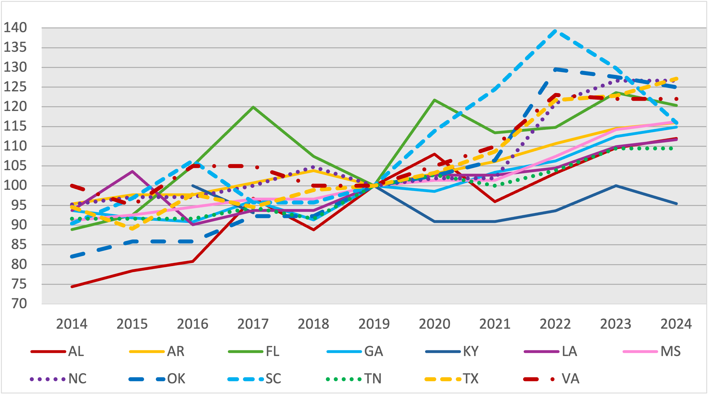
Figure 2. Index of Average Annual Cash Rents, Non-irrigated Cropland in the Southeastern U.S. (2019 = 100).

Land rental agreements between landowners and producers will vary. There are fixed cash rent agreements where an agreed upon annual rate is paid by the producer to the landowner. There are flexible cash rent agreements where some of the burden of risk is taken upon by the landowner if production costs and revenues fluctuate. In a flexible cash rent agreement, the annual rate can differ from year to year, depending upon the state of the local farm economy. There are also share agreements that exist where a portion of the production from the rented land is shared between the landowner and producer. Landowners and producers should work to find the ideal agreement that is best for both parties.
References:
U.S. Department of Agriculture (USDA) National Agricultural Statistics Service, Cash Rents Survey, August 2024. https://quickstats.nass.usda.gov/results/E0F5EB36-3313-3D7B-9E7F-E56A3365CF2B#9A9F55D7-E267-38C6-ACB9-DF106291B5A7
Smith, Amanda. “Cropland Rents.” Southern Ag Today 5(16.1). April 14, 2025. Permalink