U.S. inflation has eased from its 2022 highs, with the Consumer Price Index (CPI) stabilizing around 2.4% at the end of 2025. While the pace of price increases has slowed, elevated costs for services, housing, and food persist, maintaining pressure on consumers (see Figure 1). Inflation is expected to remain below 3% into 2026. In a Southern Ag Today article, Kim and Yoon (2025) explained why the perception of grocery inflation remains high. Despite inflation slowing, prices rarely return to previous levels; rather, they increase at a more sustainable, yet still elevated, pace. The key to offsetting increases in consumer prices is income growth. When income does not rise in line with prices, consumers lose purchasing power. To address this and ensure that households are not caught in a financial trap, several practical strategies can be considered. I have seen the suggestions below applied in real life while growing up and continue to practice them myself.
First, it is important to track household spending each month and ensure that it does not exceed total income earned. There are simple ways to do this, such as keeping a spreadsheet of all expenses as they occur. Households can also be managed like a business to ensure that “profits” (savings) are generated. These savings can then be placed in high-interest-earning accounts. A simple 80/20 budgeting rule can be applied, where 80% of income is allocated to needs and wants (rent, food, utility bills, travel, and entertainment), with needs prioritized, and the remaining 20% allocated to savings or debt repayment, if applicable.
If living expenses consistently exceed income or you are unable to meet your savings goal, analyze spending categories such as food and discretionary expenses. This analysis can help identify areas where habits can be adjusted to seek more affordable alternatives. For example, instead of eating out at restaurants, which may include not only the cost of the meal and tax, but also tips, service charges, and/or delivery fees, consider preparing home-cooked meals. This option is not only healthier but also potentially at least three times less expensive (Bachmann, 2024). Additionally, consider brewing coffee at home instead of purchasing a $6 cup daily; this can lead to monthly savings of over $100. Cooking at home also offers social benefits, such as strengthening bonds with household members and enhancing overall family well-being.
Bachmann, Kirk. “2024 Consumer Dining Trends: How Americans are Spending on Restaurants and Takeout.” Auguste Escoffier School of Culinary Arts. September 25, 2024. Accessed: February 13, 2025. https://www.escoffier.edu/blog/world-food-drink/consumer-dining-trend-statistics/.
Kim, Ashley Jiyoon, and Sungeun Yoon. “Why Grocery Inflation Still Feels High.” Southern Ag Today 5(6.5). February 7, 2025. https://southernagtoday.org/2025/02/07/why-grocery-inflation-still-feels-high/.
In January 2026, the Texas Agricultural Cooperative Council (TACC) held their annual Farm Store Summit. The Summit is a gathering of farm store managers which allows for the sharing of ideas, success stories, and strategies in response to their greatest challenges. As participants discussed the challenges facing their farm store operations, three themes stood out.
I. Increasing Competition
Consolidation in supply markets, especially for fertilizer, chemical, and seed, is having a negative impact on form store profitability. Agricultural industries are populated by some very large suppliers who may also be competitors in the retail space. That’s a difficult situation for a local cooperative farm store. Increasing urbanization adds to the challenge with a change in the surrounding customer base. As agriculture loses acres to homes and other industries, cooperatives are challenged to adapt to an urban consumer to help maintain sales volume. They strive to tell these customers that they are welcome at the co-op. These changes also bring increased competition from urban-focused retailers like Walmart, Home Depot, and Tractor Supply Co. Although cooperatives feel they might have an advantage in expertise, their competitors are marketing and distribution powerhouses.
II. Finding Good Employees
Several times during the summit a manager praised the value of a good employee. In a retail business, employees can make all the difference. They are the first to greet customers and the last to ensure that all expectations were met. Employees that are friendly and engaging with customers generate increased sales. Likewise, poor employees can leave customers feeling dissatisfied and inclined to take their business elsewhere. Even when everything else in the cooperative is executed perfectly, negative behavior and attitudes of employees will be felt in sales. As one manager put it, “culture can edge out competency”. Cooperative farm store managers are replacing the negative energy of poor employees with the profitability that comes with employees that value and understand excellent customer service.
III. The Attitude of the Board
Perhaps the greatest challenge to the cooperative farm store comes from within the board room. Many managers expressed concern over the attitude of board members toward retail operations. Board members sometimes see their farm store as a needed service rather than a profit center for the cooperative. They are willing to take losses on an activity that represents a convenience or perceived security, especially when the cooperative has another primary activity, such as a grain elevator. However, a profitable farm store represents added resilience to overall cooperative operations. Additionally, board members may focus on the convenience aspects of carrying certain inventory and neglect the profit considerations of inventory turnover. A tractor part may seem invaluable for an occasional emergency, but inventory that sits on the shelf for ten years has already lost money. Retail space and the money used to stock the shelves are investments.
Successful farm stores are valuable to their members and communities. Not only do they provide needed products and services, but they also generate profits from other parts of the supply chain. Their success depends on adapting to competition, excellent customer service, and direction from a board that is focused on profit and financial stability.
Consumers are interested in native plants (i.e., those present prior to European settlement) with heightened demand in recent years. Interestingly, positive perceptions of native plants are widespread but spending in the U.S. is uneven, with heightened spending among a relatively small group of consumers. Using a 2022 national survey of 2,066 U.S. households that purchase plants, consumer spending patterns reveal a clear segmentation story relative to native plant purchasing behavior. Consumers can be divided into three segments based on their perceptions of native plants: Native averse (32% of the sample), native curious (36%), and native enthusiast (32%). Approximately 20% of the sample (n=422) were from the USDA South region (i.e., Delaware, Washington D.C., Florida, Georgia, Maryland, North Carolina, South Carolina, Virginia, West Virginia, Alabama, Kentucky, Missouri, Tennessee, Arkansas, Louisiana, Oklahoma, Texas; USDA, 2021). Of the Southern participants, 25% were native averse, 42% were native curious, and 32% were native enthusiasts.
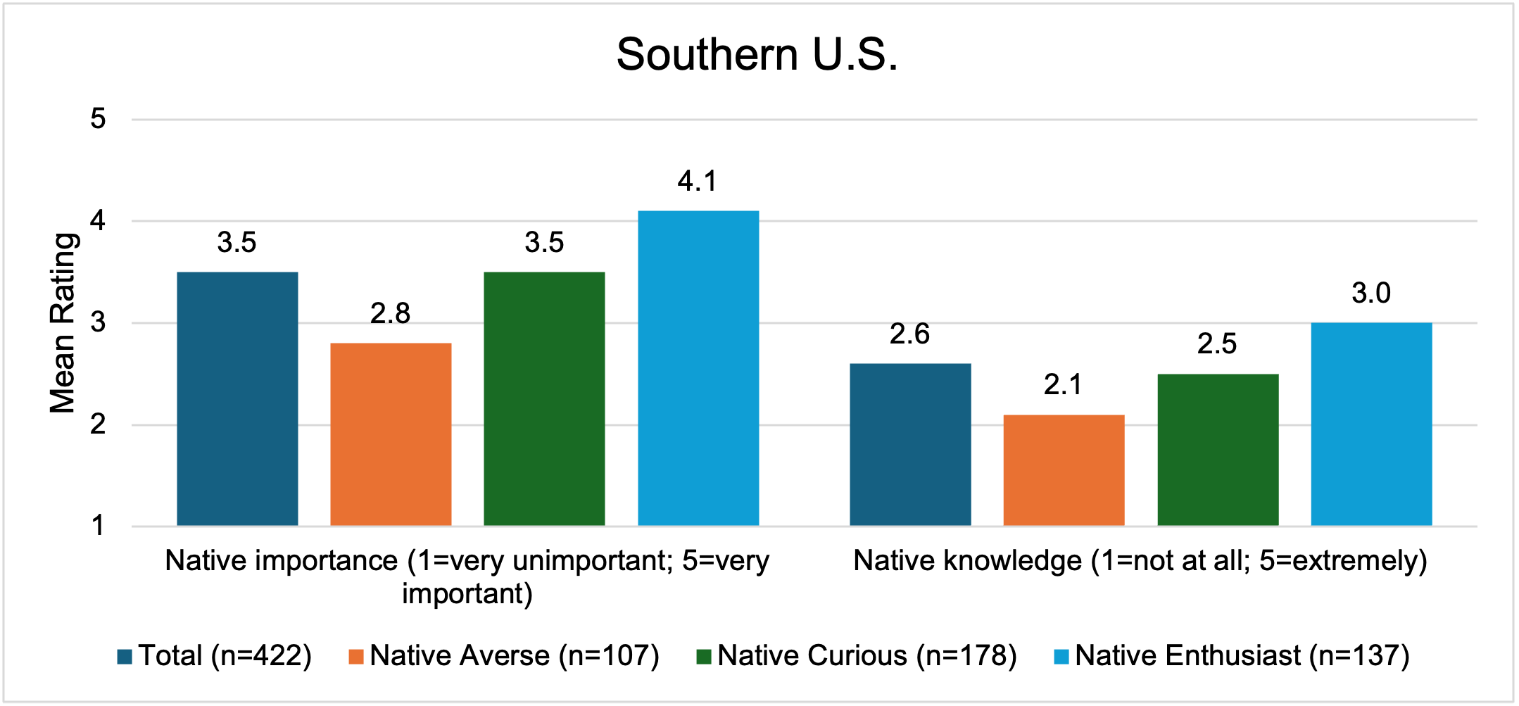
Several factors influenced segment membership including native plant perceptions, education, and plant purchasing behavior. Native enthusiasts and native curious consumers perceived native plants as providing many benefits (i.e., less maintenance, adapted to difficult sites, help water conservation, benefit the economy, improve biodiversity, are readily available, I know where to purchase native plants, are drought resistant, help pollinators, complements existing landscape, aid in natural habitat restoration, are aesthetically pleasing, and wildlife friendly) while native averse consumers did not share these perceptions. Rather, the native averse segment perceived native plants as not providing significant benefits over introduced species. The native enthusiasts also placed greater importance on native plants (in general) and reported higher subjective knowledge (Fig. 1). Similar results were observed in the U.S. and Southern region. In the South, 100% of native enthusiast members purchased native plants in 2021 (similar to 100% in the U.S. total sample), vs. 45% of native curious (46% in the U.S. total sample), and 34% of native averse segments (28% in the U.S. total sample). Education impacted segment membership, with native enthusiasts and native curious having higher education levels than the native averse group. Income did not influence segment membership, indicating that disposable income was not the driving factor behind these groupings, rather perceptions influenced subsequent plant spending behavior.
Figure 1. U.S. Consumers Perceived Importance and Knowledge of Native Plants
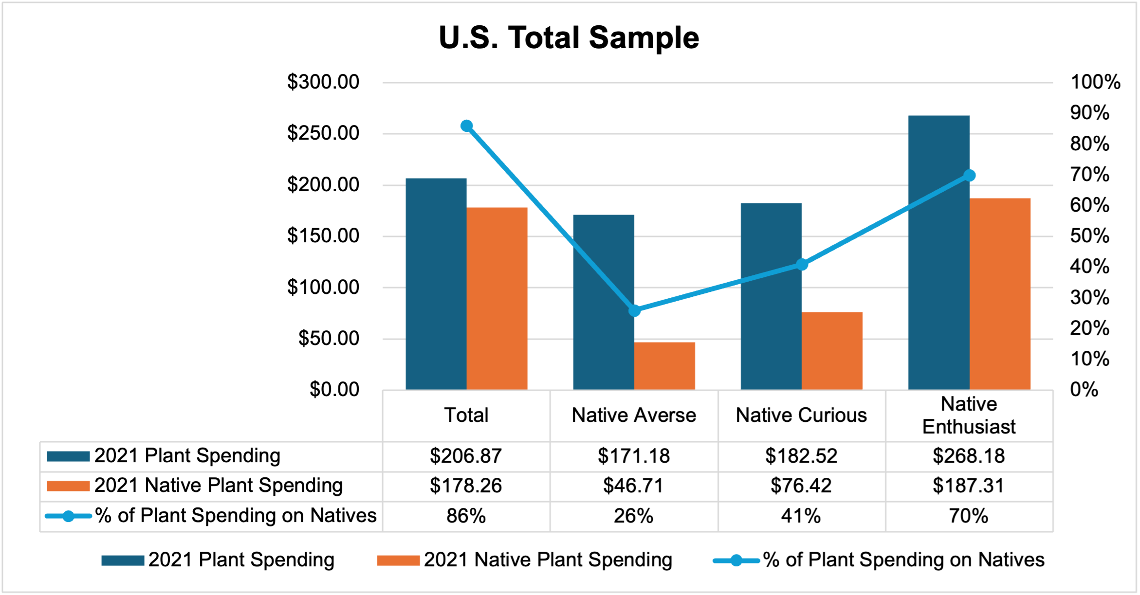
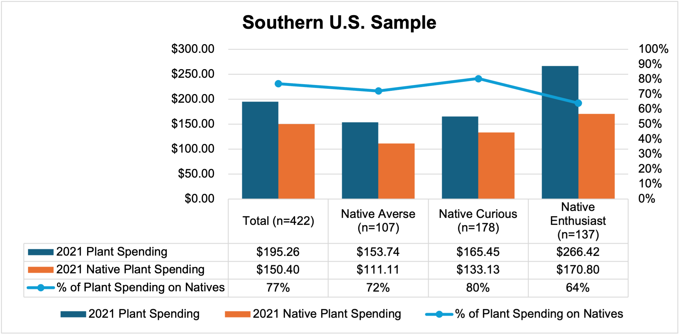
While all three segments purchase native and introduced plants, native plant expenditures are primarily driven by native enthusiasts and native curious members (Fig. 2). On average, in 2021, native enthusiasts spent $187 on native plants (70% of total plant spending), while native curious consumers spent $76 (41% of total plant spending) on native plants, and native averse spent $47 (26% of total plant spending) on native plants. In 2021 in the Southern region, native enthusiasts spent $171 on native plants (64% of total plant spending), while native curious consumers spent $133 on native plants (80% of total plant spending), and native averse spent $111 on native plants (72% of total plant spending). Of note, total plant spending was higher among native enthusiasts in both the total and Southern samples relative to the native curious and native averse which were not significantly different. This implies that the native enthusiast segment is spending more on plants in general and are likely seeking out native plants when they are available.
Figure 2. U.S. Consumer Native and Introduced Plant Spending Behavior In 2021 (n=2066).
These patterns point to potential growth in native plant sales through increasing per-customer spending among consumers who already buy plants and view native plants favorably. A small shift in the native curious consumers’ plant budgets to purchase more native plants could generate a sizable gain in total native plant sales because of the size of the segment and their receptiveness to native plants. For growers, retailers and landscapers, strategies that increase confidence in native plant selection is key. For example, clear labeling, aesthetic assortments and bundling native plants with information may be more effective than broad awareness campaigns. These strategies may be more impactful given that there is evidence that native plants are not always clearly identified at retail (Brzuszek and Harkess, 2009) and that native plants may be perceived as less desirable than introduced plants (Gillis and Swim, 2020). Thus, providing clear point-of-sale information about the plants and their benefits while demonstrating their aesthetic appeal may aid in convincing members of the native curious segment to purchase more native plants.
References:
Brzuszek RF, Harkess RL. 2009. Green industry survey of native plant marketing in the southeastern United States. HortTechnology 19:168-172. https://doi.org/10.21273/HORTTECH.19.1.168
Gillis AJ, Swim JK. 2020. Adding native plants to home landscapes: The roles of attitudes, social norms, and situational strengths. J Environ Psych. 72: 101519. https://doi.org/10.1016/j.jenvp.2020.101519
Acknowledgements: This research was supported by a grant from the Horticultural Research Institute (‘‘HRI’’). Its contents are solely the responsibility of the authors and do not necessarily represent the views of HRI.
Source: Rihn, A.L., A. Torres, B. Behe, and S. Barton. 2024. Unwrapping the native plant black box: Consumer perceptions and segments for target marketing strategies. HortTechnology. 34(3): 361-371. https://doi.org/10.21273/HORTTECH05401-24.
Rural land values in the U.S. sit at the intersection of agriculture, housing, energy, and long-term investment. Land values influence producers’ borrowing capacity and decision making while they influence households’ wealth and tax burdens, affecting the prosperity of rural communities. There was an increase in rural land and property values in the wake of the pandemic, due in part to high buyer demand. Remote workers were able to relocate from cities to rural areas as broadband access (high-speed internet) expanded and rural infrastructure improved in more remote regions (Smith, 2023), resulting in an emerging trend across the U.S. that further increased demand for rural land. Understanding the factors affecting rural land values help determine the resilience of farm operations and the affordability of rural living, both of which are important to the development of rural communities. This becomes even more pertinent given the recent shift in interest rates, along with the volatile nature of commodity prices, and growing competition for land from investors for various purposes such as renewable energy projects.
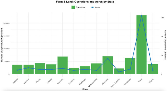
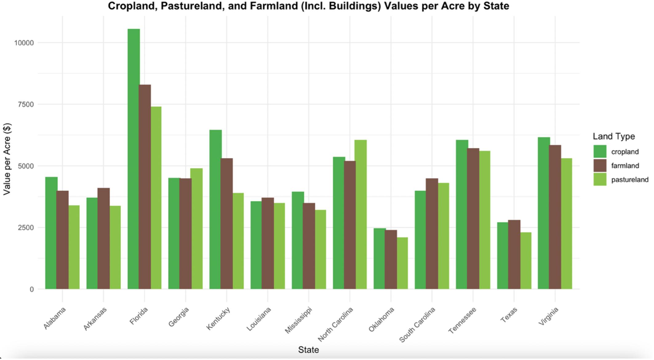
Texas is known for its rural character, having the most farmland in the country and by far the largest amount in the southern region (U.S Census, 2022, see Figure 1). Despite the state having one of the lowest land values in the region, second only to Oklahoma (Figure 2), its land value increased by about 55% over the past 10 years (Smith et al., 2025). Average per-acre land prices increased from $1,951 in 2017 to $3,021 in 2022, mostly driven by an increased recreational use potential (Smith et al., 2025). The 2024 Texas Land Trends report found that rural land values were highly influenced by demand for lifestyle-oriented buyers and investors rather than traditional farm income from production (ASFMRA-TX, 2024). Rural land in Texas was valued at nearly $300 billion in 2021, representing about 10% of the total rural real estate value in the U.S. (Su et al., 2024). Although farm income and commodity prices have shown peaks during the past decade, they have since returned to more stable levels, placing a significant financial burden on both new buyers trying to enter the market and long-time landowners struggling to hold on to their property. According to the ASFMRA- TX (2024), the strongest increases in land value in rural Texas were observed in Central Texas (48%) and the Upper Gulf Coast Region (12%) given their proximity to intense growing urban centers like Austin and Houston, respectively. In contrast, Far West Texas showed the slowest growth in value. Gilliland et al. (2020 & 2010) alluded to the sparse population, lack of urban development, and limited agricultural infrastructure as factors influencing the low land values in this region.
To examine the factors that influence land values, this article uses Washington County in Texas as an example. The county is in the Blackland Prairies region of southeast central Texas, an area influenced by its proximity to urban centers and its availability to those markets. Specifically, a 250-acre case study property was examined. The site features hilly topography, a mix of wooded and open areas, recreational infrastructure, and five building improvements, including a main house overlooking a small lake. To analyze the property’s market value and the factors influencing it, data from 136 comparable property sales in the county were used. A simple regression analysis was performed to identify significant factors that influenced land prices. The variables used in the analysis to determine the factors that influence property values in Washington County were minutes to Brenham (urban center), percentage of surface water, percentage of floodplain, percentage of wooded area, plot size, and market conditions.
The variables found to have a statistically significant impact were reduced drive time to Brenham (urban center), percentage of surface water, percentage of floodplain, and market conditions. The regression analysis showed that for every 5-minute increase in drive time to Brenham, land value decreased by 12%, while each 0.5% increase in surface water coverage added 5% to property value. Similarly, properties with more floodplain coverage saw a reduction in value by 4% for every 5% increase in floodplain, reflecting the risk for recreational buyers. Market conditions showed that land values are rising at about 1% per month, highlighting the constant rising demand. A characteristic that is important to note is that land size was deemed statistically insignificant, reinforcing the idea that amenities and accessibility influence more than acreage in recreational markets.
Washington County serves as an example of how non-agricultural factors are driving rural land valuation in Texas. Multiple factors influence land values in Texas that extend from traditional farm income and production capabilities. The statistical analysis done highlights that the tract location and accessibility are the factors that influence land value the most. As land near major cities often has a market rate significantly higher than those in remote areas. In Washington County, for example, public road frontage was found to be the most significant quality for impact on land prices, reflecting the importance of development potential and easy access. Soil quality and water availability also play major roles as fertile land and reliable water sources reduce production costs and enhance productivity (ASFMRA-TX, 2024). Other than traditional agricultural uses, recreational demand has become a powerful driver of land value, especially during the pandemic in 2020, when individuals sought for a rural homesites as comfortable retreats, prioritizing lifestyle and recreation over traditional farm income (Smith, 2023). Additionally, infrastructure and government incentives shape land value by determining how a tract of land can be used and improved. Research show that non-farm factors now play a crucial role as commodity prices or farm returns, highlighting the complex nature of Texas rural land valuation (Su et al., 2025).
Understanding the key drivers of rural land value, especially in counties like Washington, has various implications for a wide range of buyers. Landowners and investors can use this information to make more informed decisions about when and where to buy, sell, or how to develop rural properties, especially as recreational demand continues to rise. Local governments and planners benefit by recognizing how access to land, water features, and proximity to urban areas influence land use trends and can proactively manage growth through development and zoning decisions. Moreover, developers can use these findings to balance the competing interests of development and land preservation, especially in high demand areas. The growing trend of recreational land and displacement from agricultural income also raises concerns for new farmers and policy makers.
Figure 2. Cropland, Pastureland, and Farmland (including buildings) Values per Acre by State, 2024
Source: USDA-NASS (2025)
References:
American Society of Farm Managers and Rural Appraisers, Texas Chapter (ASFMRA-TX). (2024). Texas rural land value trends 2024. ASFMRA Texas Chapter.
Gilliland, C. E., Greaves, S., & Su, T. (2020). Structural trends of regional Texas rural land markets. Texas Real Estate Research Center at Texas A&M University. Available at: https://trerc.tamu.edu/article/structural-trends-regional-texas-rural-land-markets-2279/ (Accessed: 11 July 2025).
Gilliland, C. E., Gunadekar, A., Wiehe, K., & Whitmore, S. (2010). Characteristics of Texas land markets — A regional analysis. Texas A&M University Real Estate Center. Available at: https://trerc.tamu.edu/wp-content/uploads/files/PDFs/Articles/1937.pdf (Accessed: 11 July 2025).
Smith, R. (2023). Southwest land values up: COVID played a role. Farm Progress. Available at: https://www.farmprogress.com/farm-life/southwest-land-values-up-covid-played-a-role (Accessed: 11 July 2025).
Smith, L.A., Lopez, R.R., Lund, A.A., & Anderson, R.E. (2025). Status Update and Trends of Texas Working Lands 1997 – 2022. Texas A&M Natural Resources Institute, College Station, TX, USA. Available at: https://nri.tamu.edu/media/y04fu4b3/status-update-and-trends-2025-full-report.pdf (Accessed: 10 December 2025).
Su, T., Dharmasena, S., Leatham, D., & Gilliland, C. (2024). Texas rural land market integration: A causal analysis using machine learning applications. Machine Learning with Applications, 18, 100604. https://doi.org/10.1016/j.mlwa.2024.100604.
Su, T., Dharmasena, S., Leatham, D., & Gilliland, C. (2025). Modeling influence of agricultural and non-agricultural factors on Texas rural land market values. In Preprints.org.
U.S. Census Bureau. (2022). Nation’s Urban and Rural Populations Shift Following 2020 Census. Available at: https://www.census.gov/newsroom/press-releases/2022/urban-rural-populations.html (Accessed: 31 December 2025).
United States Department of Agriculture, National Agricultural Statistics Service (USDA-NASS) (2025). Available at: https://www.nass.usda.gov/Data_Visualization/Commodity/index.php (Accessed: 10 December 2025).
Southern Ag Today has recently published several articles on why producers should consider joining, starting, or becoming more involved with a cooperative in their state. An annual publication from the US Department of Agriculture’s Rural Development[i] (USDA RD) offers solid financial reasons to do the same. How does a return on investment (allocated equity in the case of a cooperative) of 11.3% to 45.2% sound? It appears that cooperatives offer a distinct advantage to farmers in their state.
How Does the South Stack Up?
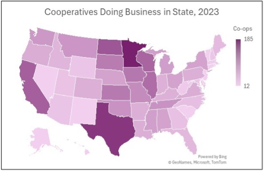
The readership might be interested in a little competition (or some light post-holiday reading) – how does the US Southern Region[ii] stack up with the rest of the US? Table 12 in the report cited above provides information on cooperatives represented in each state, which are illustrated with the heat map graphics below and ranked[iii].
Cooperatives Doing Business in Each State
Texas (#2) pulls its weight, ranking behind Minnesota in the number of cooperatives doing business in the state. Oklahoma (#11), Tennessee (12th), Mississippi (16th), and Alabama (17Th) also make the top 20.
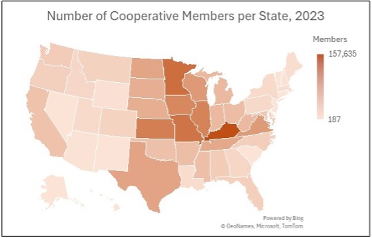
Number of Cooperative Members in Each State
Kentucky comes in first place! Virginia (#8), Texas (#9), Tennessee (#11), Arkansas (#18), Mississippi (#19), and Oklahoma (#20) combine forces to propel the Southern US into just over one-third of the top 20 placements.
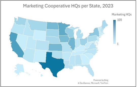
Marketing Cooperatives Headquartered in Each State
Marketing cooperatives generate their revenue from the sale of members’ products. Texas again takes the #1 spot, but only Virginia in the Southern Region makes the top 20 at #19. These results, however, may not reflect next-generation cooperatives and cooperatives organized as LLCs (i.e., peanut cooperatives in Georgia)[iv].
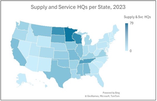
Supply and Service Cooperatives Headquartered in Each State
Supply and service cooperatives provide farmer members with what their name suggests. Southern states claim nine of the top 20 spots, with Tennessee (#4), Alabama (#6), Mississippi (#9), Texas (tied for #9), Oklahoma (#12), Arkansas (#16), Kentucky (tied for #16), Virginia (tied for #16), and Louisiana (#20).
And the Winner Is….
Honestly, anyone who is a member of a well-functioning cooperative! In terms of sheer numbers, the North Central Region is first, followed by the Southern Region in second. However, the presence of more cooperatives, their members, and specific types of cooperatives in various regions of the US is largely influenced by the types of commodities grown and the number of different commodities that can be cultivated in each region. Farm size and the density of farming operations in each location also play a role. Finally, farmers’ willingness to collaborate with other farmers seems basic, but refers to the willingness of farmers from two or three generations in the past. Many cooperatives have been around for a long time, with 78% of all cooperatives operating for more than 50 years[1].
The “well-functioning” part of a cooperative is largely due to the engagement of its members. If your farm is part of a cooperative, strive to be engaged with it by attending meetings, voting in elections, serving as a board member, and encouraging the next generation to do the same.
If you are looking to start a cooperative or improve a cooperative’s performance, many land-grant universities have specialists who help cooperatives succeed by training and developing cooperative board members and staff.
[ii] The US Southern Region, as defined by the Southern Risk Management Education Center, comprises 13 states, which account for approximately 26% of the US states (and a larger proportion of the land mass). The other regions are also defined, based on the types of crops grown in each region.
[iii] To keep things simple, this article just compares the number of states each region has in the Top 20, as the acres of farmland, number of farmers, and the volume of business through each cooperative in each region may vary significantly.
[iv] The report excludes cooperatives that deviate from the one-member, one-vote model, as well as those that handle more than 50% of their volume from non-members.