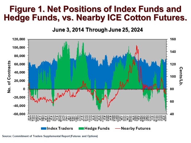
Author: John Robinson

It is important for farmers to have accurate knowledge of their costs of production.  Having a historical baseline of production costs gives producers a standard for managing their operation.  Accurate knowledge of production costs is also the basis for developing a marketing plan, i.e., identifying break-even price levels to target your price risk management or selling.

There are tools available to assist producers.  There are commercial software products that provide useful database management and financial calculations.  Some Extension agricultural economists provide support using standard accounting programs like Quickbooks.  Extension agricultural economists in major cotton producing states also publish planning budgets, often in spreadsheet formats, to guide producers in developing their own customized cost and returns estimates. Lastly, the USDA Economic Research Service (ERS) also conducts regular grower surveys of production costs, by region, and publishes research reports based on this information (Figure 1).

Figure 1 summarizes annual data on U.S. average annual cotton production costs.  The data depict two measures of historical profitability:  1) short run profitability, reflected as the value of cotton production less specified variable costs, and 2) long run profitability, calculated as the value of cotton production less specified variable and fixed costs.  The value of production shown does not include farm program payments or crop insurance indemnities.

On the face of it, these data reflect U.S. cotton as a marginal proposition.  While there appears to be an economic rationale to operate in the short run, and partially contribute to fixed costs, the long run profitability implications of U.S. cotton appear poor. The possible implications for long term viability of U.S. cotton include the following.  1) The cotton growing operations that will be left are likely of a scale that implies lower than average fixed costs, particularly machinery costs. This may involve beneficial leasing terms that are unavailable to smaller scale producers.  2)  The larger scale operations may also benefit from volume discounts on purchases of variable and capital inputs.  3) Some operations may generate above average value of production.  On the yield side, this perhaps is being achieved by the early adopters of yield enhancing technology and production systems.  On the price side this could involve better risk management and marketing that captures some of the upside price risk that is available in most years. Lastly, the picture implied by Figure 1 reinforces the need for the buffering effects of federal farm programs and crop insurance. 

Figure 1. Cotton U.S. Net Return Cost Trend

References and Resources

Beginning Quick Books Online Training for Farmers and Ranchers. https://amarillo.tamu.edu/files/2023/08/QuickBooks-Online-Course-Flyer.pdf.

Texas A&M AgriLife Extension. Cotton Budgets. https://agecoext.tamu.edu/resources/crop-livestock-budgets/by-commodity/cotton/.

University of Georgia. Department of Agricultural and Applied Economics. Budgets. https://agecon.uga.edu/extension/budgets.html.

University of Arkansas Cooperative Extension Service. Crop Budgets for Arkansas. https://www.uaex.uada.edu/farm-ranch/economics-marketing/farm-planning/budgets/crop-budgets.aspx.

USDA Economic Research Service. Commodity Costs and Returns. https://www.ers.usda.gov/data-products/commodity-costs-and-returns/.

---

Robinson, John. “U.S. Cotton Cost Trends and Implications.” Southern Ag Today 3(46.1). November 13, 2023. Permalink

For spring planted crops like cotton, a key market influence in the fall season is the refinement of the national production forecast.  U.S. cotton production forecasts are published monthly by USDA’s National Agricultural Statistics Service (NASS).  For example, the current U.S. cotton production forecast is 13.13 million bales.^[1]  The forecast is expressed in standard 480-pound bale equivalents (or statistical bales).  Actual physical bales (or running bales) tend to weigh closer to 500 pounds, so analysts typically use conversion factors following USDA, e.g., 1.0275 statistical bales for every running bale.

Acreage and Production Data. Between May and July, NASS’s forecast of cotton production is based on surveyed planted acreage and assumed historical averages for yield and abandonment. Beginning in August, the production forecast incorporates grower survey data on acreage, yield, and abandonment.  Also beginning in August, the South Texas cotton forecast incorporates data from “objective yield surveys” which involve field sampling of boll counts and weights.  In September, this field sampling expands to include all of Texas, Arkansas, Georgia, and Mississippi, with repeat monthly sampling through December.  Lastly, the production forecast is occasionally adjusted in the fall months based on crop insurance information (USDA Risk Management Agency) and/or certified acres data (USDA Farm Service Agency).

Ginnings Data.  All U.S. cotton is ginned following harvest.  Surveys of gins are performed by USDA NASS who then publishes a monthly forecast of cumulative bales ginned as of that month.  For example, the number of actual U.S. bales ginned as of September 1 was forecasted at 484,450 running bales.^[2]  This converts to 497,772 statistical bales, which is 4% of USDA’s September production forecast for this year’s crop.  This is a seasonally normal percentage of the total U.S. crop.  

Classing Data.  All U.S. cotton bales are sampled for fiber quality.  It follows that the most accurate, albeit unfolding, measure of cotton production is the cumulative count of bales classed by USDA’s Agricultural Marketing Service (AMS).  These data are reported weekly as running bales.  Through the week ending September 8, 2023, AMS reports cumulative classings of 531,866 running bales of upland cotton and no pima cotton.^[3]  This converts to 546,492 statistical bales of all cotton which, unexpectedly, exceeds NASS’s ginned bale forecast.  It is assumed that the weekly count of classed bales is always the more accurate measure.

Reconciliation/Refinement.  The ginnings and classings data are published until the conclusion of ginning season, typically in the first quarter of the year following harvest. NASS will then reconcile their production forecast with final cumulative ginning and classing numbers (the latter two being converted to statistical bales).  The effect of this reconciliation is the refining of NASS’s production forecast to its final estimate.  Figure 1 shows that August production estimates have been between 15% below and almost 20% over final estimates with a lot of variation.  Each monthly refinement in production estimates occurred until final estimates were achieved by May for the last twelve crop years (2011 through 2022).  The refinement concluded by April in eight out of the twelve crop years and was finished in March in six out of the twelve crop years.  In general, the tightening pattern of percent deviations from the final production forecast reflects the influence of the updated USDA data flow.

---

^[1]  USDA-NASS.  2023.  Crop Production 09/12/2023.

^[2]  USDA-NASS.  2023.  Cotton Ginnings 09/12/2023.

^[3]  USDA-AMS.  2023.  Cotton Weekly Quality Report by State 9/8/2023.

---

Robinson, John. “USDA Refining of Forecasted U.S. Cotton Production.” Southern Ag Today 3(38.1). September 18, 2023. Permalink

It is frequently challenging to forecast crop production because of varying local weather and crop conditions.  In the case of upland cotton, the situation is further complicated by plant biology. The major row crop substitutes to U.S. cotton include corn, sorghum, wheat, soybeans, and peanuts. The first three of these are annual grasses, while the latter are annual legumes. The reproductive strategy of these annuals is to produce as much seed (yield) as allowed by weather and soil conditions. As a result, aggregate yields of annual crops are often thought to be well correlated with weekly crop condition rates. 

In contrast, upland cotton is relatively more complicated in its growth habits and resulting predictability.  The reason is that cotton is a perennial in its native tropical environment, akin to a crepe myrtle bush.  When grown as an annual crop in temperate regions, cotton plants can still shift back and forth between vegetative and reproductive growth.  This mixed and indeterminate growth habit is illustrated by a poor visual inspection of the weekly cotton crop condition and the resulting Texas average cotton yield (Figure 1).  The Texas aggregate situation is even further complicated by the range of planting dates, from March-April in southern Texas to May-June in northwestern Texas.  Such phenomena in Texas can have a major influence on U.S. production estimates since Texas represents over half of U.S. planted acreage (USDA NASS). 

The situation in 2023 is further complicated by a mid-year shift in the weather.  The first quarter of 2023 saw severe drought conditions over much of Texas (Figure 2, left panel).  Widespread and repeated rains since April have reportedly helped developing crops in southern Texas while complicating planting in northwestern Texas.  How much the latter will contribute to more or less cotton production is unknown. It is possible that the State will realize prevented planting from drought preceding prevented planting from too much rain.  With much of the growing season still ahead, further shifts in weather may also occur.  It may not be until early fall before we have reliable forecasts of the resulting production outcome.

Figure 1. Texas Cotton Crop Condition Index

Figure 2. U.S. Drought Monitor Maps from March 7, 2023, and June 6, 2023

---

Robinson, John. “Difficulty in Forecasting 2023 U.S. Cotton Production.” Southern Ag Today 3(24.1). June 12, 2023. Permalink

The USDA February 2023 Cotton Outlook projects world cotton consumption bottoming at 110.7 million bales for the current 2022/23 marketing year.  They then forecast 2023/24 consumption recovering to 115.5 million bales due to: 1) post-Covid reopening in China with increasing GDP, 2) lower Chinese production and greater need for Chinese imports, and 3) an “unusual inventory dynamic” of pent-up cotton demand following previously Covid-disrupted deliveries of cotton textile goods.  Other bullish influences for cotton consumption include the competitively low prices of raw cotton, which appear to have translated to higher levels of U.S. cotton exports since January.

Beyond China, world GDP is also currently forecasted by the International Monetary Fund to rise slightly to 2.9% (Figure 1, dashed green line).  This is important to the cotton market because cotton consumption tends to rise with economic growth and fall with economic declines.  For example, the blue line in Figure 1 shows world cotton consumption ranging between about six and eight pounds per person per year.  The peaks and valleys of per capita cotton consumption coincide with the respective trends of world GDP.  This is not surprising since cotton-made apparel and home furnishing products are both semi-durable and somewhat discretionary.  

Growing expectations of stronger economies, increasing mill use, and stronger export demand are, in turn, bullish influences on ICE cotton futures.  In the near term, they could contribute to stronger old-crop prices, especially if the current hedge fund net short position is liquidated in a short covering rally.

There are, of course, counter influences. First, a bullish demand response would be somewhat self-correcting as mills generally buy less cotton at higher prices. It remains to be seen how long and how high the “unusual inventory dynamic” will push cotton prices.  In addition, there is a potential macro-economic risk shrinking the demand curve and putting downward pressure on prices.  The latter could result from strong recessionary influences due to high interest rates as central banks continue their attempt to lower inflation to target levels.  

Figure 1. World Per Capita Cotton Use and Global Economic Growth

---

Robinson, John. “Competing Influences and Expectations for World Cotton Demand.” Southern Ag Today 3(16.1). April 17, 2023. Permalink

Photo by Pixabay: https://www.pexels.com/photo/full-frame-shot-of-cracked-pattern-255509/

U.S. cotton production is typically uncertain in any given year, in part because roughly half the acreage is in Texas.  Still, the 2023 season is starting off with a more than usual degree of uncertainty.

First, the early season forecasts of U.S. cotton plantings vary by as much as two million acres, i.e., from 9.5 to 11.5 million acres.  Such a discrepancy puts a premium on the milestone planting intentions reports from the National Cotton Council (released February 12) and USDA (March 31 Prospective Plantings report and June 30 Acreage report).

The weather is a second major source of variability.  The National Oceanic and Atmospheric Administration’s Climate Prediction Center (CPC) is forecasting a transition from the hotter/drier La Niña condition to a neutral influence by late Spring.  CPC further predicts the onset of the cooler/wetter El Niño condition by early Fall.  That’s all well and good, but there is uncertainty around all weather forecasts.  Will the beginning dryness lead to above average early season abandonment?  Or will neutral El Niño-Southern Oscillation (ENSO) conditions by planting time surprise us with timely planting rains and good growing conditions?

The third consideration is whether the recent signs of improving cotton demand will continue.  There is plenty of uncertainty about whether the broader economy is recovering or entering a double dip recession.  

These three variable situations outline some possible extremes.  If, for example, U.S. cotton growers plant a low level of acreage, and it continues dry, and abandonment is above average, and demand continues to recover, the result could be ending stocks below 3 million bales.  Historically, it suggests that Dec’23 futures might follow the seasonal path of the green line in Figure 1, strengthening as the growing season goes on.  In the context of this year’s price levels, it suggests a march back up through the 90s towards a dollar.

On the other hand, what if 11+ million acres are planted and receive timely rains?  That could lead to three million more bales of production than the first scenario.  If demand doesn’t recover enough to absorb these bales, the carryover outcome could be five or six million bales.  In years of building excess stocks, the historical seasonal average of December ICE futures reflects weakening prices.  The pattern of the blue line in Figure 1 could push prices under 80 cents.

Figure 1’s red line reflecting “Stable Carryover” years is simply the in between scenario, with middling implications for ending stocks and prices. The level of these seasonal averages isn’t as important as the pattern itself.  Time will tell how all these variables play out.  

Figure 1. December Futures Seasonal Average Price in Stable, Larger and Smaller Carryover Years

Author: John Robinson

Professor and Extension Economist

---

Cotton Photo by Mark Stebnicki: https://www.pexels.com/photo/plantation-of-cotton-in-a-cropland-10287687/

Robinson, John. “Possible Extreme Outcomes for 2023 Cotton.” Southern Ag Today 3(7.1). February 13, 2023. Permalink