The European Deforestation Regulation (EUDR) has been postponed once again for another calendar year, but effects of the regulation are already being seen with Southern agricultural and timber lands. Forestland owners in the south are being told they may need to sign an attestation stating they will not convert their timberland to pasture or row crop production after timber is harvested. Failure to sign the attestation may bar a landowner from selling their timber if that product could end up in the European Union (EU). Because many larger timber and paper companies do business with the EU, this regulation could greatly limit the number of potential timber buyers in a geographical area or eliminate them entirely.
The EUDR is a regulation passed by the EU back in May 2023. The stated goal of the regulation is to reduce the EU’s impact on global deforestation and degradation by prohibiting the importation into the EU of certain products produced on land deforested or degraded after Dec. 31, 2023.
The products of importance to southern agriculture consist of wood, cattle, and soybeans. Companies importing these goods to the EU will need to certify that their products do not contribute to deforestation or degradation of forested lands. Companies that are in violation of the new regulation are subject to potentially stiff financial penalties, including confiscation of the product being sold, up to 12 months of exclusion from the EU public procurement process, and fines up to 4% of the company’s total annual EU turnover from the preceding year after the fine is assessed. With penalties this large at stake, companies are looking for ways to comply with the EUDR, and the burden is being shared with southern landowners.
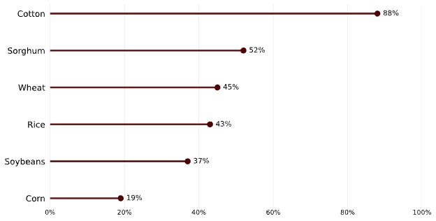
A substantial share of U.S. agricultural production is sold overseas (Figure 1). Exchange rates, therefore, play a central role in export competitiveness and, indirectly, in domestic price prospects. For crops with heavy export exposure, the value of the dollar is not just a macroeconomic headline; it is part of the demand curve faced by Southern producers.
The economic intuition is straightforward. Most globally traded agricultural commodities are priced in U.S. dollars. When the dollar strengthens, foreign buyers must use more local currency to purchase the same dollar-priced commodity, which tends to soften demand at the margin and place downward pressure on prices. When the dollar weakens, U.S. supplies become cheaper in foreign-currency terms, export bids often improve, and U.S. crops become easier to place in global markets. This helps explain why the dollar and broad commodity prices frequently move in opposite directions, even though exchange-rate effects can be offset by other market forces.
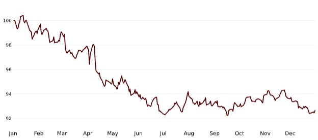
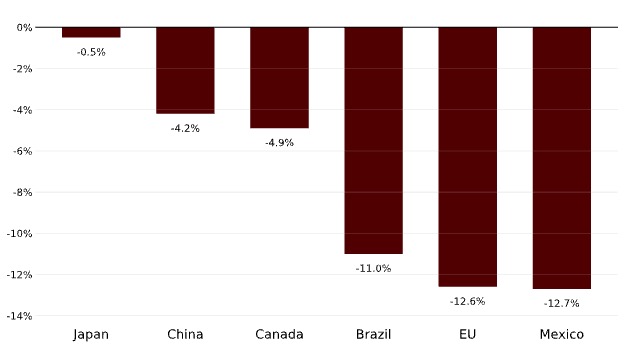
In 2025, the exchange-rate environment turned more supportive for U.S. agriculture. After rising 7.1 percent in 2024, the nominal broad dollar index declined 7.2 percent over 2025 (Figure 2). Over the same period, major U.S. agricultural customers experienced notable currency appreciation against the dollar: the euro strengthened 12.6 percent, and the Mexican peso appreciated 12.7 percent (Figure 3). These movements improved foreign purchasing power for U.S. shipments and helped support U.S. crop exports. At the same time, Brazil’s real appreciated by roughly 11 percent, which can tighten Brazilian exporters’ local-currency margins and reduce their ability to price aggressively, all else equal.
Empirical research supports this channel. Shane et al. (2008) find that a 1 percent decline in the trade-weighted dollar is associated with roughly a 0.5 percent increase in the value of U.S. agricultural exports. Exchange rates, however, rarely operate in isolation. Weather outcomes, yields, freight costs, geopolitics, and policy shocks can dominate price formation in the short run (an important lesson from the post-2022 period).
For Southern producers, the dollar’s decline in 2025 is a constructive signal for export-oriented crops because it supports international competitiveness without requiring lower farm-gate prices. The main limitation is timing: exchange-rate effects pass through bids, basis, and contracting practices unevenly, so benefits can vary across regions and marketing windows. Even so, the directional effect is favorable.
If global conditions remain orderly and U.S. interest rates drift lower, the dollar may stay softer and continue to support the export channel; renewed risk aversion, however, could reverse this trend and reintroduce headwinds. For export-dependent Southern crops, monitoring exchange-rate conditions alongside basis and contract timing remains an essential part of marketing discipline.
Figure 1 – Exports account for a large share of output in several U.S. crops
Note: Export share is calculated as exports divided by total production. Estimates correspond to USDA 2025/26 marketing-year projections released in January 2025. Source: U.S. Department of Agriculture, World Agricultural Supply and Demand Estimates (WASDE), January 2025
Figure 2 – The U.S. dollar declined in 2025
Note: Nominal Broad U.S. Dollar Index, Index 2025-01-02=100, Daily, Not Seasonally Adjusted. A decline indicates a broad-based depreciation of the U.S. dollar against major trading partners. Source: Federal Reserve Bank of St. Louis (FRED): DTWEXBGS
Figure 3 –U.S. dollar weakened against key agricultural trading partners in 2025
Note: Percent change over 2025 (end-to-end). Exchange rates are expressed as local currency per U.S. dollar (Negative values indicate a weaker U.S. dollar). Source: Federal Reserve Bank of St. Louis (FRED): DEXBZUS, DEXCHUS, DEXMXUS, DEXCAUS, DEXJPUS, DEXUSEU. For the Euro, we convert FRED’s DEXUSEU (USD per EUR) to EUR per USD as 1/DEXUSEU
References
Federal Reserve Bank of St. Louis. (2026). Federal Reserve Economic Data. FRED. https://fred.stlouisfed.org/. Accessed January 23, 2026
U.S. Department of Agriculture, Office of the Chief Economist. (2025, January). World Agricultural Supply and Demand Estimates (WASDE). https://www.usda.gov/oce/commodity/wasde. Accessed January 23, 2026.
In 2025, U.S. peanut planted area reached its highest mark since 1991, at 1.95 million acres, as was confirmed by the recently released Crop Production Annual Summary. This increase in peanut acreage was driven by a 70,000-acre jump in Georgia and a 45,000-acre increase in Texas. Mississippi was the only major peanut-growing state that had a decrease in peanut planted area compared to 2024. At the end of the 2025 growing season, 97.6% of the area planted was harvested, which was the highest rate since 2014.
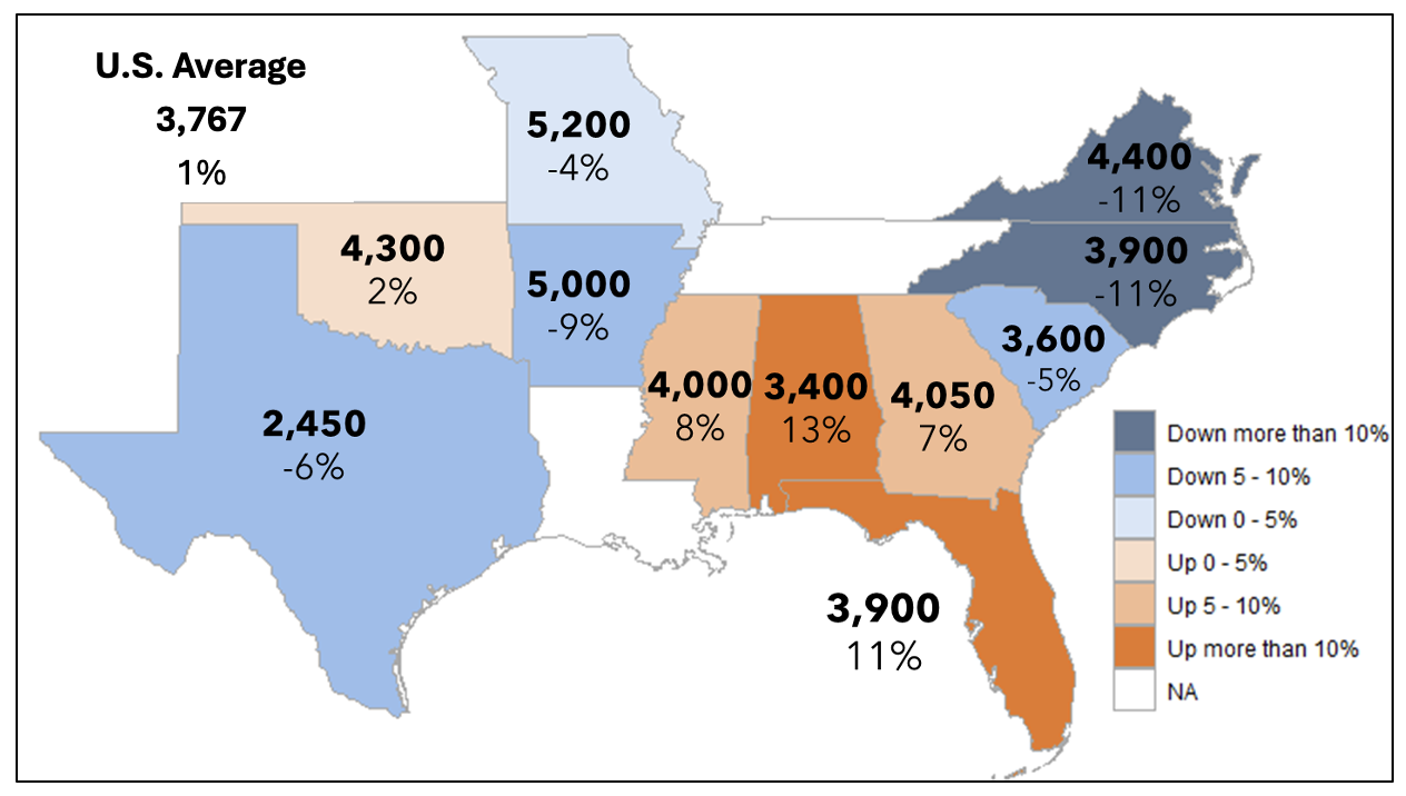
Figure 1: 2025 Peanut Yield by State (lb./acre) and Percent Change from 2024
Data source: USDA-NASS. 2025Crop Production Annual Summary.
The U.S. had a middling peanut yield, averaging 3,767 lb. per acre (Figure 1). While this yield was 1% higher than 2024, it falls about 130 lb. per acre below the previous five-year average. Georgia – the leading producing peanut state – averaged 4,050 lb. per acre, which marks a 7% increase from last year’s value, but still 12% below the high in 2012. Alabama, Florida, and Mississippi observed similar yield increases. Oklahoma had a small increase of just 2%, but the second-highest yield on record for the state. In contrast, Texas had a significant decrease in yield, at 2,450 lb. per acre, the smallest state yield since 1995, when Texas farmers produced 2,000 lb. per acre.
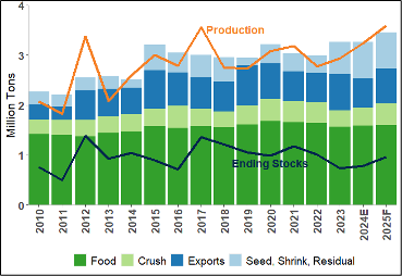
Figure 2: Peanut Production, Disappearance, and Ending Stocks by Year
Data Source: USDA-ERS. Oil Crops Outlook: January 2026.
Overall, peanut production was lower than expected by about 110 thousand tons from what was forecast in September (Rabinowitz, 2025). However, at an estimated 3.59 million tons in 2025, total production was still up 11%, and edged out the 2017 total of 3.56 million tons for the highest on record (Figure 2). While total peanut disappearance is forecast to increase 6% for the 2025-26 marketing year, it is expected to fall short of production, leading to a 24% increase in ending stocks. As we look into 2026, peanut prices are lower than last year, but competing crops’ prices are not looking any better. Corn prices are slightly lower than they were last year in mid-January, with September futures prices down to around $4.40 per bushel. December cotton futures are in the 68-cent-per-lb range, similar to this point last year. As a result, I expect that we will see another sizeable peanut planted area in 2026.
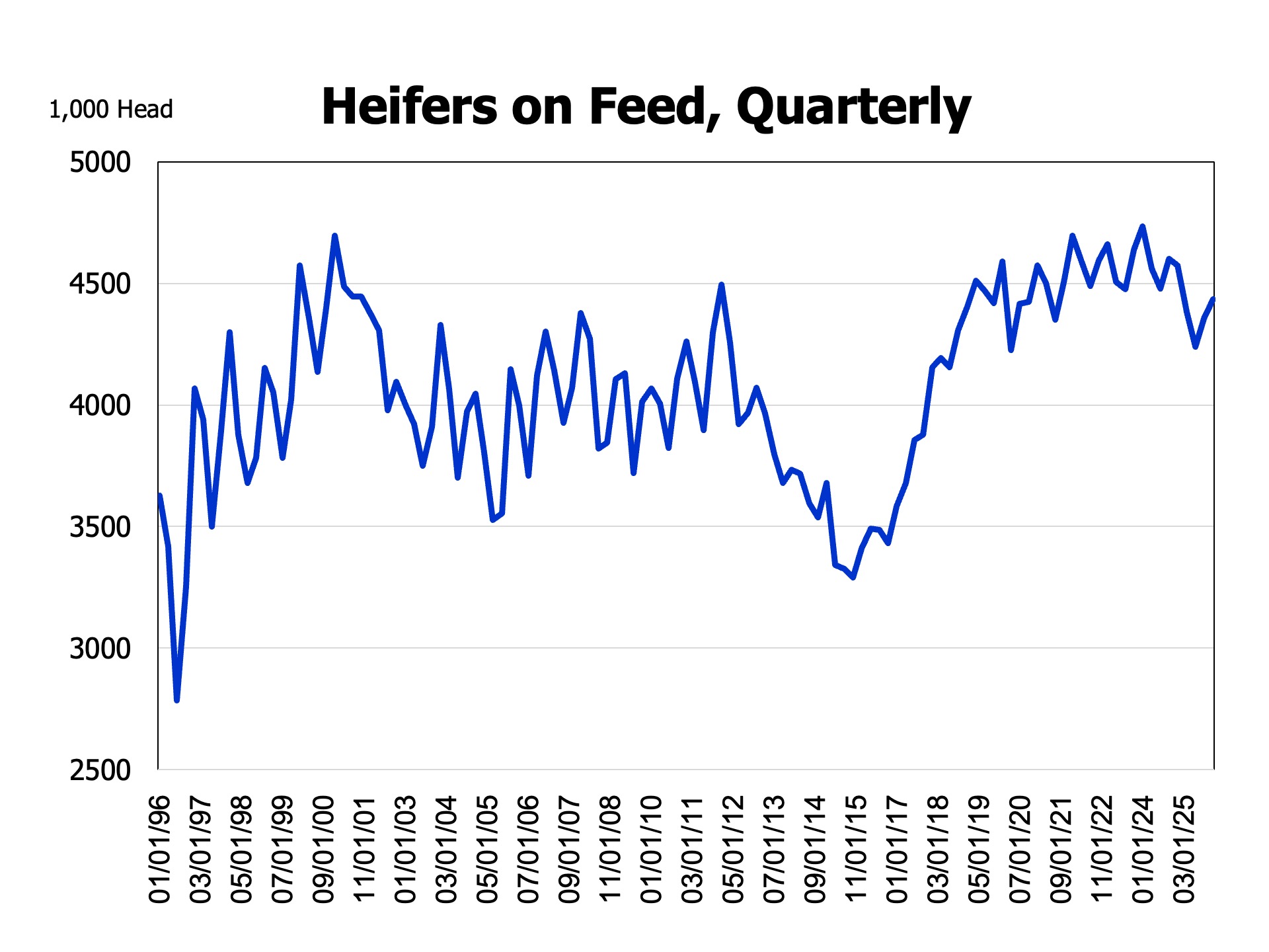
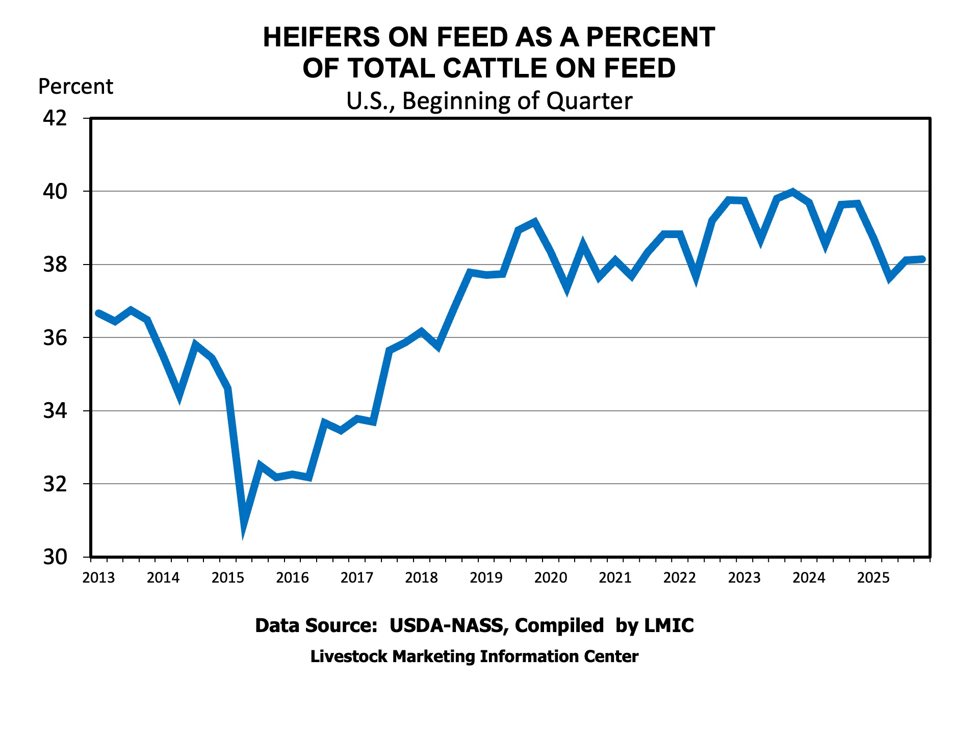
USDA’s Cattle on Feed Report, released on Friday, January 23rd, contained the estimated number of heifers on feed. The breakout of steers and heifers on feed is released quarterly. Many have been looking closely at this statistic for evidence of a significant herd expansion starting.
Heifers on feed totaled 4.435 million head, down 140,000 head, or 3.1 percent, from last January 1. The number of steers on feed also declined by 3.2 percent. Heifers represented 38.73 percent of the total cattle on feed, hardly different from last year’s 38.70 percent. It was the fewest January 1 heifers on feed since 2019. Arizona, Colorado, Oklahoma, and Texas had fewer heifers on feed, with Colorado having the largest decline of 85,000 head, followed by Texas, down 55,000 head. The decline in the heifers on feed in those states is interesting in that those states would have been most impacted by the border closure with Mexico. Other states either reported no change or, in the case of Nebraska, 10,000 more heifers on feed.
Spayed heifers imported from Mexico contribute to the total number of heifers on feed. The January Cattle on Feed report is the first full month of comparison to a year ago, with no cattle imports in December 2025 and 2024. Approximately 145,000 fewer spayed heifers were imported from Mexico in the months leading up to January 1, 2026, compared to January 1, 2025. So, the decline in heifers on feed could largely reflect fewer imports rather than a significant decline in domestic heifer feeders being placed.
While the decline in heifers on feed suggests some heifers held for herd rebuilding, the reduction in supplies from Mexico and heifers as a percent of all cattle on feed indicates little herd rebuilding from additional domestic heifer retention, yet. It is likely that the inventory report released on the 30th should indicate more heifers held for beef cow replacement.
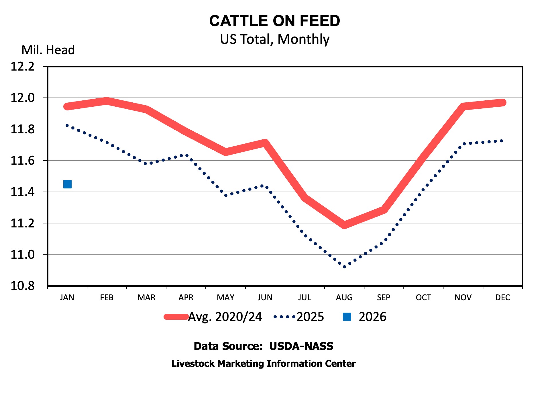
The rest of the cattle on feed largely lined up with expectations. Marketings were up about 2 percent, with one more slaughter day during December, daily average marketings were below a year ago. Placements were 5.4 percent below a year ago. The total number of cattle on feed was down 3.2 percent a year ago. Supplies should continue to tighten this year and into next year, as well.
In the fourth quarter of 2025, average pine sawtimber stumpage prices across the South softened further. Pine sawtimber averaged $23.23/ton, about 6% lower than a year ago and 10% below its early-2022 peak (TimberMart-South, 2026). Pine chip-n-saw prices remain relatively stable at $17.50-18.20/ton, essentially unchanged from last year but roughly 20% below 2022 levels. Pine pulpwood prices continued to slide, averaging $5.96/ton, down 22% year over year and 46% below their 2022 peak. Hardwood pulpwood prices held around $8/ton, stable over the past two years but still 33% lower than 2022 levels. Hardwood sawtimber prices remained relatively stable at $33.55/ton.
Figure 1. Average pine sawtimber stumpage prices by state and subregion, Q4 2025
Data source: TimberMart-South (2026)
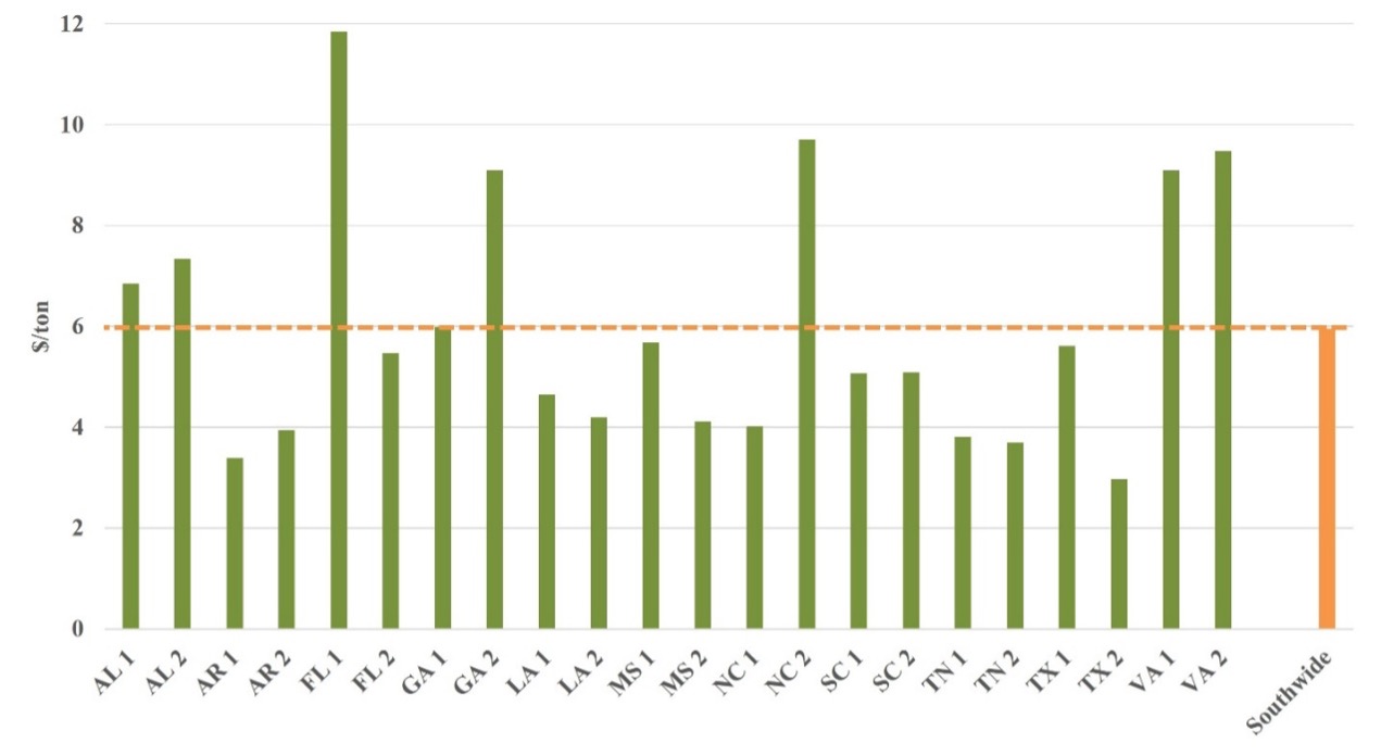
In Q4 2025, pine pulpwood prices ranged from below $4/ton in Arkansas, Southern Louisiana, Tennessee, and Southeast Texas to $9-14/ton in North-Central Florida, South Georgia, Eastern North Carolina, and Virginia (Figure 2). Compared to a year ago, prices declined sharply in South Georgia (-40%), South Carolina (-32%), Arkansas (-27%), and Louisiana (-26%), while remaining relatively stable in Alabama, Mississippi, and Tennessee.
Figure 2. Average pine pulpwood stumpage prices by state and subregion, Q4 2025
Data source: TimberMart-South (2026)
A closer look at southern timber markets
Weaker pine sawtimber prices reflect softness in the housing market. Over 70% of the U.S. softwood lumber and structural panel consumption is tied to single-family construction and remodeling activity (Alderman, 2022). While new single-family homes now account for a larger share of for-sale inventory than before the pandemic, overall supply remains constrained by affordability challenges, higher construction and financing costs, labor shortages, zoning restrictions, and rising existing homes for sale. In October 2025, single-family housing starts fell 7.8% year over year to a seasonally adjusted annual rate of 874,000 units (U.S. Census Bureau, 2026).
Tariffs on Canadian softwood lumber have increased sharply since August 2024, with total duties now reaching 45.16%. While these higher tariffs may support U.S. production over the long term, they are likely to increase construction costs in the short run and further constrain housing starts.
Reflecting weaker lumber demand, lumber mill utilization rates declined from 81% in Q2 2021 to 68% in Q3 2025 (U.S. Census Bureau, 2025). Several major lumber producers have announced deeper curtailments and downtime to better align output with market conditions.
The continued decline in pine pulpwood prices reflects ongoing structural changes in the pulp and paper industry, including product shifts, increased use of recycled fiber, mill modernization, and relocation to lower-cost regions. These trends intensified in 2025, reducing regional demand for pulpwood and placing downward pressure on stumpage prices (Figure 3). Between 2023 and 2025, more than 10 major pulp facilities in the South closed, removing over 25 million tons of annual fiber demand and significantly reshaping regional pulpwood markets.
In areas heavily impacted by Hurricane Helene, storm-related salvage further compounded these effects, leading to sharper price declines. Conversely, new investments and mill expansions in South Alabama and Arkansas have increased local demand and helped support pulpwood prices in those areas.
Figure 3. U.S. South wood-using pulping capacity, 2014-2025
Data source: Forisk (2025)
Looking Ahead
Single-family building permits, a leading indicator of housing starts, fell to 876,000 units in October, 9.4% lower than a year earlier (U.S. Census Bureau, 2026). Although Federal Reserve interest rate cuts in 2025 may ease financing conditions, housing starts are expected to remain under pressure in 2026. Remodeling and repairing activity, however, is projected to continue slow but steady growth (JCHS, 2025; NAHB, 2026). Higher tariffs on Canadian lumber may provide modest support demand for domestic production.
Overall, pine sawtimber prices in the South are expected to remain relatively stable. Areas heavily damaged by Hurricane Helene may face tighter timber supply and upward pressure on sawtimber prices due to inventory losses, particularly where growth-to-drain ratios were already low (USDA Forest Service, 2024). Pulpwood prices are expected to continue trending downward in most areas through 2026, though prices may remain stable locally where new investments add demand.
References
Alderman, D. 2022. U.S. forest products annual market review and prospects, 2015-2021. General Technical Report FPL-GTR-289. Madison, WI.
Forisk. 2025. Forisk North American forest industry capacity database. Athens, GA: Forisk.
JCHS. 2025. Leading Indicator of Remodeling Activity (LIRA). Cambridge, MA.
NAHB. 2026. NAHB/Westlake Royal Remodeling Market Index (RMI).