Southern Timber Market Update
In the fourth quarter of 2025, average pine sawtimber stumpage prices across the South softened further. Pine sawtimber averaged $23.23/ton, about 6% lower than a year ago and 10% below its early-2022 peak (TimberMart-South, 2026). Pine chip-n-saw prices remain relatively stable at $17.50-18.20/ton, essentially unchanged from last year but roughly 20% below 2022 levels. Pine pulpwood prices continued to slide, averaging $5.96/ton, down 22% year over year and 46% below their 2022 peak. Hardwood pulpwood prices held around $8/ton, stable over the past two years but still 33% lower than 2022 levels. Hardwood sawtimber prices remained relatively stable at $33.55/ton.
Stumpage prices varied widely across states and subregions. In Q4 2025, pine sawtimber prices ranged from about $17-21/ton in Tennessee, South Carolina, and Alabama to over $30/ton in Florida and North Carolina (Figure 1). Timber prices are inherently local, influenced by mill demand, weather, accessibility, timber quality, species mix, and local inventories. Compared to a year ago, pine sawtimber prices rose moderately in North Georgia (+20%) and North-Central Florida (+14%), declined in South Carolina (-26%), Northeast Texas (-16%), Alabama (-19%), and North Carolina (-12%), while remaining relatively stable elsewhere.
Figure 1. Average pine sawtimber stumpage prices by state and subregion, Q4 2025

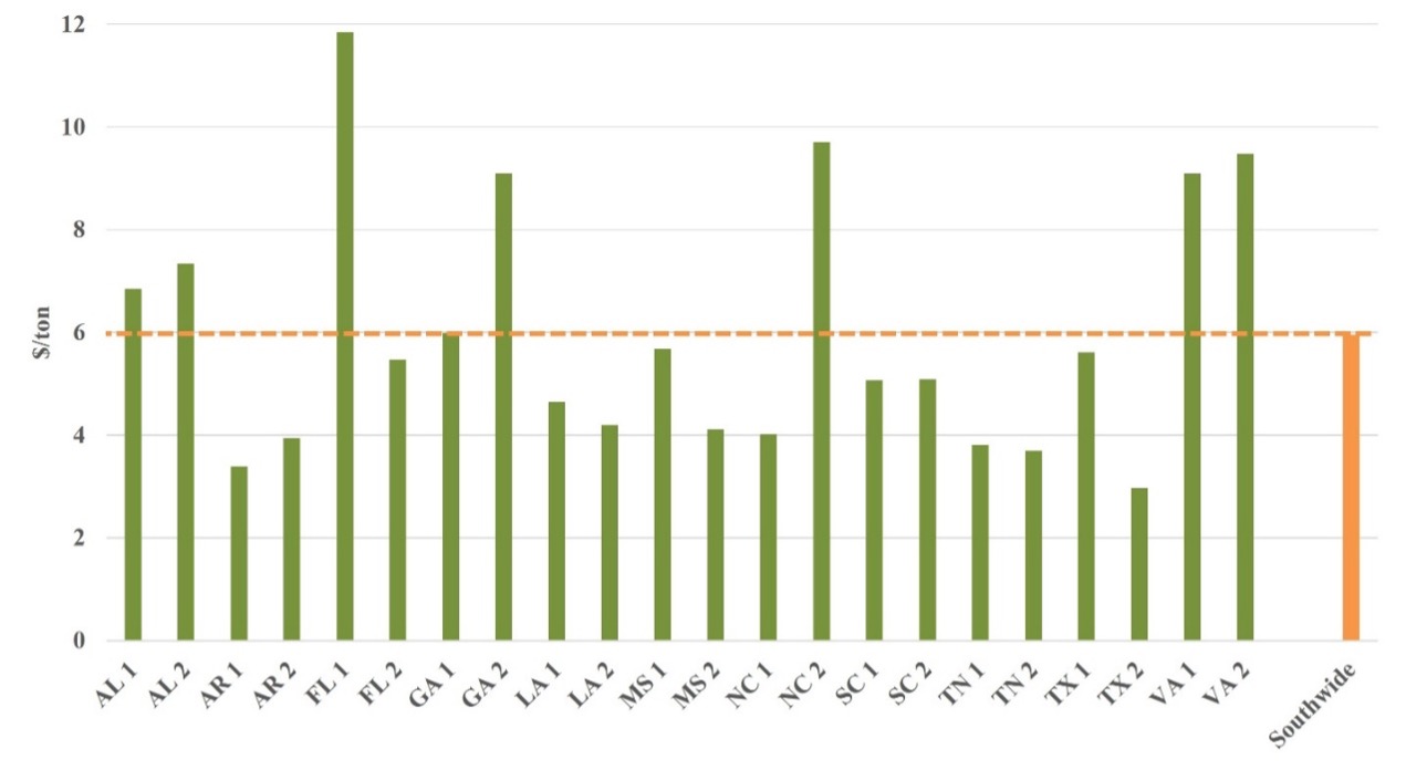
In Q4 2025, pine pulpwood prices ranged from below $4/ton in Arkansas, Southern Louisiana, Tennessee, and Southeast Texas to $9-14/ton in North-Central Florida, South Georgia, Eastern North Carolina, and Virginia (Figure 2). Compared to a year ago, prices declined sharply in South Georgia (-40%), South Carolina (-32%), Arkansas (-27%), and Louisiana (-26%), while remaining relatively stable in Alabama, Mississippi, and Tennessee.
Figure 2. Average pine pulpwood stumpage prices by state and subregion, Q4 2025
A closer look at southern timber markets
Weaker pine sawtimber prices reflect softness in the housing market. Over 70% of the U.S. softwood lumber and structural panel consumption is tied to single-family construction and remodeling activity (Alderman, 2022). While new single-family homes now account for a larger share of for-sale inventory than before the pandemic, overall supply remains constrained by affordability challenges, higher construction and financing costs, labor shortages, zoning restrictions, and rising existing homes for sale. In October 2025, single-family housing starts fell 7.8% year over year to a seasonally adjusted annual rate of 874,000 units (U.S. Census Bureau, 2026).
Tariffs on Canadian softwood lumber have increased sharply since August 2024, with total duties now reaching 45.16%. While these higher tariffs may support U.S. production over the long term, they are likely to increase construction costs in the short run and further constrain housing starts.
Reflecting weaker lumber demand, lumber mill utilization rates declined from 81% in Q2 2021 to 68% in Q3 2025 (U.S. Census Bureau, 2025). Several major lumber producers have announced deeper curtailments and downtime to better align output with market conditions.
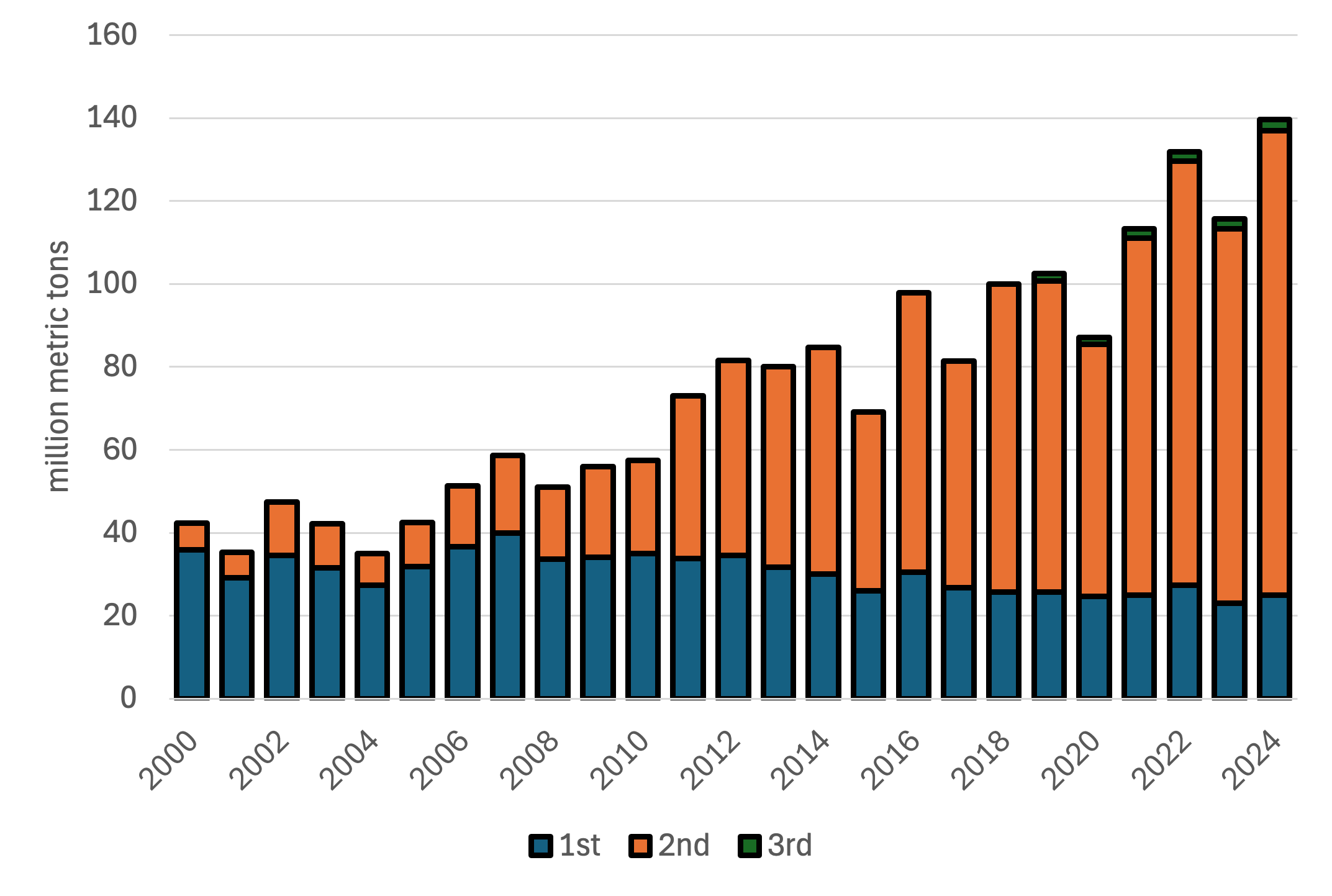
The continued decline in pine pulpwood prices reflects ongoing structural changes in the pulp and paper industry, including product shifts, increased use of recycled fiber, mill modernization, and relocation to lower-cost regions. These trends intensified in 2025, reducing regional demand for pulpwood and placing downward pressure on stumpage prices (Figure 3). Between 2023 and 2025, more than 10 major pulp facilities in the South closed, removing over 25 million tons of annual fiber demand and significantly reshaping regional pulpwood markets.
In areas heavily impacted by Hurricane Helene, storm-related salvage further compounded these effects, leading to sharper price declines. Conversely, new investments and mill expansions in South Alabama and Arkansas have increased local demand and helped support pulpwood prices in those areas.
Figure 3. U.S. South wood-using pulping capacity, 2014-2025

Looking Ahead
Single-family building permits, a leading indicator of housing starts, fell to 876,000 units in October, 9.4% lower than a year earlier (U.S. Census Bureau, 2026). Although Federal Reserve interest rate cuts in 2025 may ease financing conditions, housing starts are expected to remain under pressure in 2026. Remodeling and repairing activity, however, is projected to continue slow but steady growth (JCHS, 2025; NAHB, 2026). Higher tariffs on Canadian lumber may provide modest support demand for domestic production.
Overall, pine sawtimber prices in the South are expected to remain relatively stable. Areas heavily damaged by Hurricane Helene may face tighter timber supply and upward pressure on sawtimber prices due to inventory losses, particularly where growth-to-drain ratios were already low (USDA Forest Service, 2024). Pulpwood prices are expected to continue trending downward in most areas through 2026, though prices may remain stable locally where new investments add demand.
References
Alderman, D. 2022. U.S. forest products annual market review and prospects, 2015-2021. General Technical Report FPL-GTR-289. Madison, WI.
Forisk. 2025. Forisk North American forest industry capacity database. Athens, GA: Forisk.
JCHS. 2025. Leading Indicator of Remodeling Activity (LIRA). Cambridge, MA.
NAHB. 2026. NAHB/Westlake Royal Remodeling Market Index (RMI).
TimberMart-South. 2026. Market news quarterly. Athens, GA.
U.S. Census Bureau. 2025. Quarterly survey of plant capacity utilization. https://www.census.gov/programs-surveys/qpc.html
U.S. Census Bureau. 2026. Monthly new residential construction, October 2025. https://www.census.gov/construction/nrc/index.html
USDA Forest Service. 2024. Forest Inventory Analysis Program Forest Inventory EVALIDator web-application. St. Paul, MN.
Li, Yanshu. “Pine Sawtimber Prices Soften as Pine Pulpwood Continues to Fall.” Southern Ag Today 6(5.1). January 26, 2026. Permalink