Row-crop producers across the South faced another difficult year in 2025. Weather challenges led to wide yield variability across much of the region. Even where yields were strong, low commodity prices and persistently high input costs kept margins tight, leaving many operations near or below breakeven for a third straight year. Shifts in acreage were common, with corn gaining ground at the expense of cotton and, in some areas, soybeans.
Financial stress remains a major concern heading into 2026, as limited storage capacity, tighter credit conditions, and low prices continue to pressure farm profits. To capture conditions across the south, we asked Extension agricultural economists in each state to provide a brief summary of the 2025 season. Their state-by-state perspectives are below.
Alabama – Adam Rabinowitz, Max Runge, and Wendiam Sawadgo, Auburn University
Alabama’s row crop producers faced the wettest May on record statewide, leading to delayed or prevented crop planting across the state. Prevented plantings for upland cotton in 2025 totaled 62,000 acres, above the previous five-year average of 2,000 acres. Across all crops, prevented plantings totaled 122,000 acres, much higher than the 22,000-acre five-year average. Compounding issues during the season were a late drought that suppressed peanut and soybean performance and the cotton jassid (two-spotted leafhopper) that entered Alabama and spread to all cotton-producing parts of the state. Even with these challenges, corn and cotton yields are projected to exceed their five-year averages, whereas peanut and soybean yields are expected to finish near historical norms. Meanwhile, producers, lenders, and agribusinesses remain concerned about the ongoing price squeeze driven by low commodity prices and elevated production costs. For the year ahead, many are questioning the best direction for row crops with no positive change to prices or input costs expected, and the unknown future and impact of the cotton jassid (two-spotted leafhopper).
Arkansas – Ryan Loy, Hunter Biram, and Scott Stiles, University of Arkansas
Arkansas row crop producers entered the 2025 crop year in one of the most financially challenging environments of the past decade, as crop receipts fell by $465 million to $4.46 billion, marking the third consecutive annual decline. Corn led the downturn with a 31% year-over-year decline, followed by soybean and rice receipts, while cotton receipts remain soft due to acreage reductions. At the same time, production expenses remain elevated relative to historical averages, with fertilizer, seed, labor, and interest costs continuing to pressure operating margins. Across all principal crops, state-average net returns are projected to be negative, with breakeven prices and yields often 30–40% above expected levels; late planting from generational flooding in April further increased downside risk. Record ad hoc assistance through ECAP and SDRP is expected to exceed $1 billion and offset a portion of these losses. Yet, net farm income for the crop sector is still projected to remain negative even after accounting for program payments. The mounting financial strain facing Arkansas producers continues as they confront low commodity prices, persistently high input costs, and tighter credit conditions.
Florida – Kevin Athearn, Amanda Phillips, and Joel Love, University of Florida
Florida planted acres of peanuts were up 7% (175,000 acres), corn down 3% (85,000 acres), and cotton down 29% (62,000 acres) in 2025 relative to the 5-year average (USDA-NASS). Estimated yields for peanut were up 8% (3,900 lbs/acre) and cotton up 23% (800 lbs/acre) relative to the 5-year average (USDA-NASS). Anecdotally, irrigated corn yields were above average, but non-irrigated corn yields suffered from insufficient summer rainfall. Peanut contracts were offered on a relatively small portion of production at $500 to $525 per ton, but uncontracted peanuts reportedly were selling below $400 per ton at harvest. The local basis on grain corn forward contracts offered by three Florida buyers, April through July for August delivery, averaged $0.80 over Sep futures. Forward contracts on Florida cotton typically are tied to December futures, which averaged 66.83¢ per pound between April and November. Production costs, especially machinery, labor, and interest, have trended upward, and the local UAN28 price increased 30% in early 2025. Sample budgets for 2025 estimated contribution margins per acre (not including land or fixed costs) of about $300 for irrigated peanut, $50 for irrigated corn, negative $100 for irrigated cotton, and negative $50 for non-irrigated cotton. The estimated gross profit was negative for all three crops.
Georgia – Amanda Smith, University of Georgia
The 5-year average crop mix in Georgia consisted of 44% cotton, 28% peanuts, 16% corn, 7% wheat, and 5% soybeans. Row crop producers faced another tough year in 2025, after a difficult 2024 where they incurred negative to small margins and dealt with the aftermath of Hurricane Helene, which destroyed one-third of the cotton crop, delayed peanut harvest, and damaged infrastructure. Due to cotton prices below cost of production in 2025, producers made a major shift to their crop mix by planting more peanuts than cotton for the first time in three decades and significantly increasing corn acres. The 2025 crop year saw 35% of total acres planted to peanuts, 32% to cotton, 21% to corn, and 6% each to soybeans and wheat. Despite some relief provided by government programs (ECAP and SDRP), producers continued to deplete their working capital and erode equity, making it necessary to rely on other sources of income to support their row crop operations. The 2025 crop year saw an additional challenge with the rapid spread of a new invasive pest to cotton, the Cotton Jassid (two-spotted leafhopper). Late-season drought made dryland peanut harvest difficult and created some concern about crop quality. For 2026, producers will be mindful of crop rotations and cost of production while hoping to hold on until improved agricultural policies provide needed financial relief.
Kentucky – Grant Gardner, University of Kentucky
Three consecutive years of lower prices have already put Kentucky producers in a difficult position, and this year’s extreme yield variability is adding even more pressure. Some areas will post record yields, while others will fall well below average—especially soybeans, which are currently rated in the worst condition of any state. A major concern right now is the lack of soybeans in storage. At harvest, many producers moved beans rather than storing them due to uncertainty surrounding the trade dispute, leaving most available storage filled with corn. That decision removed the opportunity to take advantage of last month’s rally in soybean futures, and many producers were unable to benefit from the price improvement when it finally arrived. While diversified operations with livestock may still be close to break-even, row-crop-focused farms are likely hovering at or below break-even for the third consecutive year, tightening cash reserves and leaving many operations increasingly vulnerable to financial stress or potential default.
Louisiana – Michael Deliberto, Louisiana State University
In Louisiana, corn acres increased by 330,000 acres (+75%) from 2024 to 2025. Most producers favored corn over cotton (and, to a lesser extent, soybeans) due to grain price competitiveness. Overall, yields were near the previous four-year average of 176 bushels per acre. Prices are finally becoming somewhat favorable for producers who elected to store their crop.
Like most of the mid-south region, cotton acres in Louisiana were down year-over-year. Producers planted only 90,000 acres in 2025. Despite the low acreage, yields were at record highs at 1,314 pounds per acre, nearly a 250-pound-per-acre increase from the previous year. While yields were excellent, prices remained low. The high cost of production, coupled with the narrow price movement within the 66-68 cents per pound range in the spring, was a main factor behind the reduced acreage in the state.
Soybean acres in Louisiana were down year-over-year. Acreage for the oilseed is typically between 1.1 and 1.2 million acres. However, the 2025 acreage was 790,000, mainly due to lackluster prices and trade uncertainty surrounding exports. Yields were the highest in five years, coming in at 54 bushels per acre.
Rice acres in Louisiana totaled 482,000 planted acres in 2025, the most since 2010. The yield per acre was 6,650 pounds, which is on par with the five-year average. High production costs and decreasing rice prices at harvest presented a major challenge for rice growers heading into the winter.
Mississippi – Will Maples, Mississippi State University
Weather played a major role in Mississippi’s 2025 crop. Frequent heavy rains delayed planting for many producers, and late-summer drought stressed crops, resulting in significant yield variability across the state. Soybeans remained the largest crop at 1.8 million acres, but growers shifted more toward corn than cotton, planting 900,000 acres of corn compared with 330,000 acres of cotton. Financial conditions remain difficult. The price environment is still unfavorable, and because Mississippi producers harvest early and lack the storage capacity common in other states, many were unable to capitalize on the recent soybean price rally. High production costs continue to squeeze margins, leaving most producers facing negative profits for the third consecutive year. Looking ahead to 2026, a growing number of producers have expressed equity concerns as they evaluate their farm financing options.
North Carolina – Nicholas Piggott, North Carolina State University
In North Carolina, 2025 row-crop outcomes were mixed. Corn yields rebounded sharply from last year’s drought-reduced crop, with NASS estimating 139 bu/acre, pushing corn production up about 75% from 2024. Late-November cash bids for No. 2 yellow corn are mostly $4.60 at country elevators and around $4.80 at feed mills, with a firm basis of $0.40-$0.50. Soybean yields, by contrast, slipped to about 36 bu/acre, below last year’s 39 bu/acre, leaving statewide soybean production down roughly 6% from 2024. Cash soybean bids are currently in the $10.50–$11.10/bu range at elevators and $11.25 at processors, with basis typically -$0.30 at elevators and $0.02 at processors. On wheat, growers have responded to several years of weak prices and weather risk by cutting back acreage: NASS reports 2025 winter wheat seedings at about 350,000 acres, down from 410,000 acres last year and near the low end of the historical range for the state. Looking Ahead to 2026 – North Carolina growers should carefully pencil out expected corn and soybean margins when making planting decisions for 2026, and pay close attention to wheat growing conditions in the next few months since they will shape production levels, basis strength, and marketing opportunities for 2026.
Tennessee – Aaron Smith, University of Tennessee
In Tennessee, 2025 row production was highly variable. Drought during July and August reduced yields and contributed to a second consecutive season of losses for many corn, soybean, and cotton farmers. Cotton and soybean yields were hardest hit by the drought and will likely result in further downward revisions from current USDA yield estimates. High input costs, low commodity prices, and below trend yields resulted in per-acre losses between $100 and $250 for many producers. Before crop insurance and other government payments, Tennessee corn, cotton, soybean, and wheat farmers are projected to lose over $400 million in 2025. With substantial year-over-year losses, many producers will carry operating debt over into the next season for the second straight year. Obtaining credit for the 2026 crop will be challenging for many producers without ad hoc government payments. Canola acres in Tennessee and Kentucky continued to expand in the fall of 2025, providing producers with an alternative to more traditional double-cropping systems. Growth in canola acreage has been driven by contracted acres, primarily in Northwest Tennessee, to support a pilot program to produce sustainable aviation fuel.
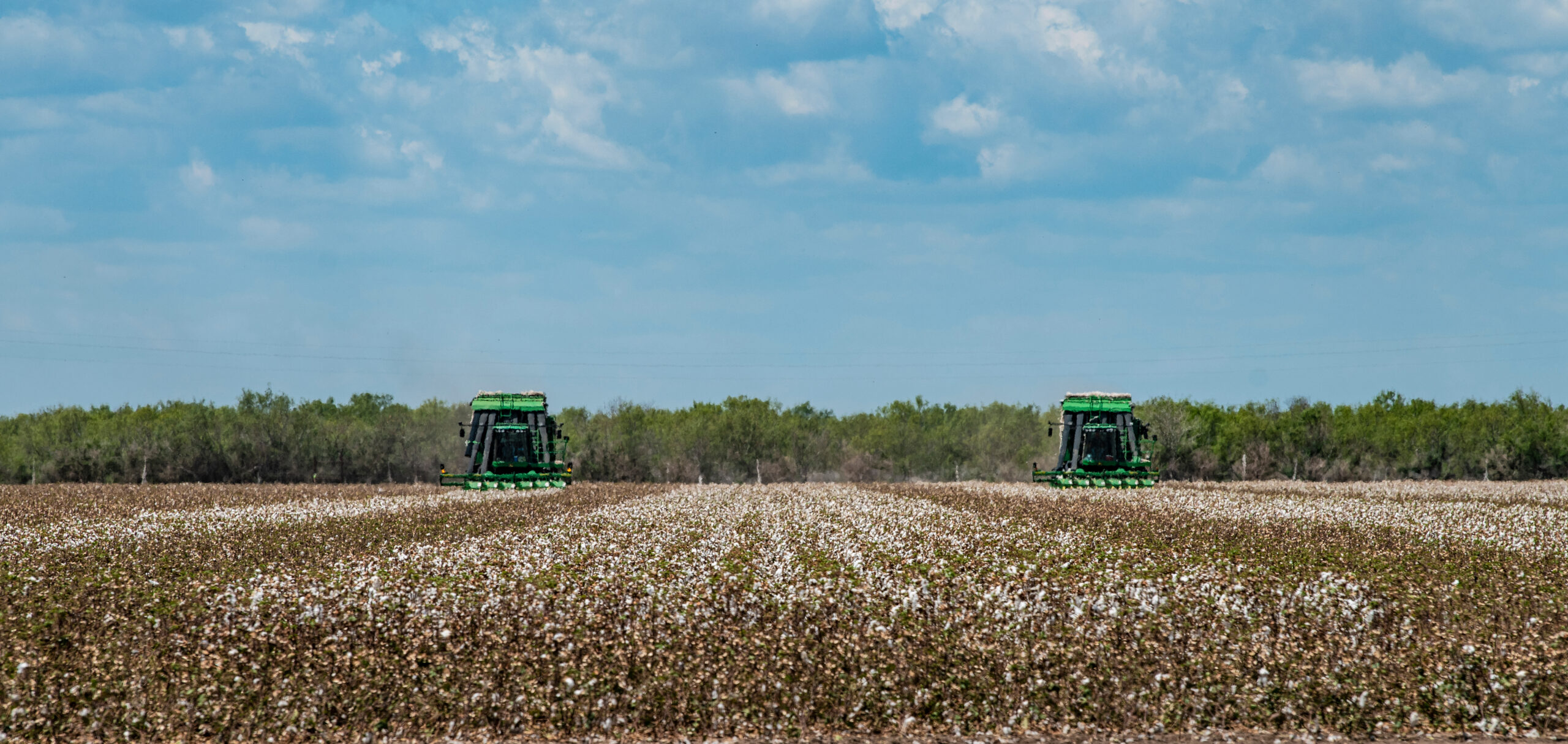
Texas – Mark Welch and John Robinson, Texas A&M University
Grain production across Texas in 2025 was generally an improvement from 2024. Overall, yields for wheat, corn, and grain sorghum were above their most recent 10-year averages. Cash grain prices for the year peaked in February and followed a decline throughout the growing season. A major feature of planning for 2026 will be changes to the farm safety net compared to the beginning of last year: a higher level of support in programs administered by the Farm Service Agency (FSA) and increased cost-sharing for crop insurance products. This could make higher levels of revenue protection a viable consideration for the upcoming crop year.
Texas cotton production in 2025 benefited from favorable, timely moisture conditions. This is in contrast to the preceding three years, which suffered from excessive heat and dryness. Unfortunately, the 2025 cotton production still suffered from unprofitably low market prices. The upcoming 2026 cotton season is concerning with a return of dry conditions and an uncertain market outcome.