USDA’s National Agricultural Statistics Service’s (NASS) Census of Agriculture is published every five years and provides data at the U.S., state, and county levels. One metric tracked is the average age of agricultural producers. This information is provided for selected southern states for the Census reporting periods 2017 to 2022, along with the percentage change in average age for that timeframe.
The overall average ages for all producers for 2017 and 2022 for the southern states are indicated in Table 1. In all states, average producer ages were increasing. For 2022, Mississippi and Florida had the highest average ages of producers at 59.6 and 59.5 years old, respectively. Georgia, Kentucky, and Tennessee had the largest percent change increases in average ages from 2017 to 2022. North Carolina had no change.
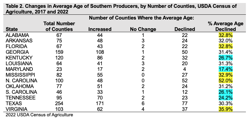
For this same timeframe, North Carolina had the largest numbers of counties with declines in average age of producers for 52 of their 100 counties, or 52 percent, followed by Virginia, Mississippi, Alabama, and Florida (Table 2). Those with the smallest include Maryland, Tennessee, South Carolina, and Kentucky.
Figure 1 depicts county level decreases (yellow shade) or increases (blue shade) in average age of producers for the states analyzed. Those counties with no changes are depicted in a red hatched fill.
Figure 1. County Level Change in Average of Age of Producers from 2017 to 2022 Census
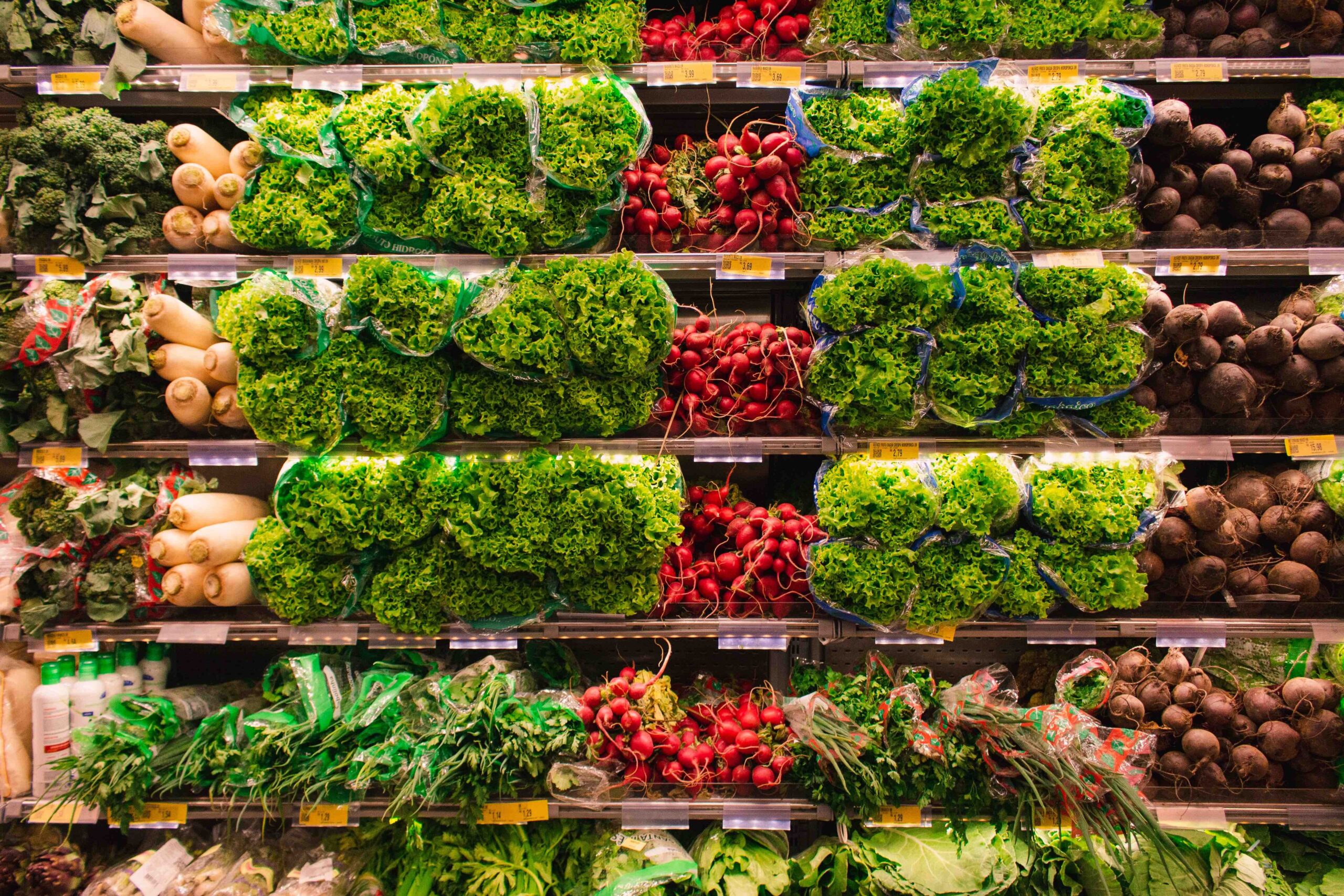
In a previous article titled Challenges for U.S. Fruits and Vegetables we discussed some of the challenges that the U.S. fruit and vegetable industry faces. Labor cost and availability is identified as the main challenge that the U.S. fruits and vegetable industry faces. Dependance on foreign-born farm labor is around 70 percent. Therefore, in order to address the shortage of farm labor, the H-2A Temporary Agricultural Program—often called the H-2A visa program— was created in 1986.
The H-2A provides a legal means to bring foreign-born workers to the United States to perform seasonal farm labor on a temporary basis, for a period of up to 10 months. Employers in the H-2A program must demonstrate, and the U.S. Department of Labor must certify, that efforts to recruit U.S. workers were not successful. Employers must also pay a State-specific minimum wage rate, which may not be lower than the average wage rate for crop and livestock workers surveyed in the Farm Labor Survey (FLS) in that region in the prior year, known as the Adverse Effect Wage Rate (AEWR). Figure 1 shows the AEWR by state and it is obvious that those rates are much higher than the federal minimum wage as well as any state minimum wage. In addition, H-2A employers must provide transportation, housing, food, insurance, and visa application fees, among other expenses that could add between 35% to 40% of the AEWR rate, i.e., $21.77 in Texas, $20.68 in Florida and $27.65 in California. Industry experts shared that agricultural wage rates in Mexico averages around $20.59 in Colima and $23.53 in Sonora per day, or $2.57 and $2.94 per hour for an 8-hour workday, respectively. Finally, as the labor shortage keeps getting worse, producers could be getting into wage bidding wars to secure farm labor during peak season, increasing their labor cost even more.
Even though labor cost takes a major toll on the fruits and vegetable industry, it is left with little to no options. Not only is the share of the labor cost higher than other agricultural industries, but also labor is scarce. According to ERS (2023), one of the clearest indicators of the scarcity of farm labor is the fact that the number of H-2A positions requested and approved has increased more than sevenfold in the past 17 years, from just over 48,000 positions certified in fiscal 2005 to around 371,000 in fiscal year 2022. The average duration of an H-2A certification in fiscal 2022 was 5.65 months, implying that the 371,000 positions certified represented around 175,000 full-year equivalents. A certified job does not necessarily result in the issuance of a visa; in fact, in recent years only about 80 percent of jobs certified as H-2A have resulted in visas. Around 300,000 visas were issued in fiscal 2022 by the Department of State.
Foreign Agricultural Service (FAS). Global Agricultural Trade System (GATS). Online database. https://apps.fas.usda.gov/gats/default.aspx. Online public database accessed February 2024.
Payment limitations are not a novel policy tool. Modern day limits have been imposed since the 1970 Farm Bill, with multiple changes to the payment limit in subsequent farm bills (Congressional Research Service, 2020; Ferrell, Fischer, Lashmet, 2024). We provide an example of what incentivizes a producer to create a new entity to receive potentially forgone commodity program payments and how it could be completed in practice when appropriate. It should be note that there are rules in place that prohibit farmers from restructuring just to avoid payment limits.
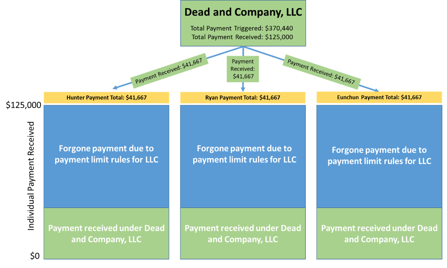
Suppose a producer is one of three members (with equal ownership shares) of Dead and Company, LLC, located in Lawrence County, Arkansas. The entity has 2,800 acres of long grain rice base; the county average Price Loss Coverage (PLC) payment yield is 63 cwt/ac[1], and the payment rate is $2.10/cwt. This would result in a total PLC payment for Dead and Company, LLC of $370,440[2]. However, under current rules, Dead and Company, LLC is subject to a $125,000 payment, and each member is also subject to a personal payment limit of $125,000, however, based on their one-third share they are limited to $41,667. In this example, Dead and Company, LLC receives the full $125,000 payment limit, effectively forgoing $245,440 ($81,813 per member) of the total payment. A visual example is provided in Figure 1 below.
Figure 1. Example of Payment Limit Distribution and Forgone Payment under an LLC
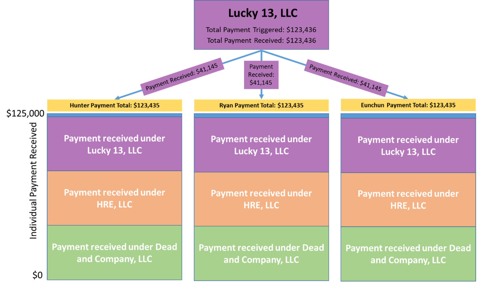
If it makes sense within the operation of the business, the three members of Dead and Company, LLC could choose to reallocate the 2,800 base acres to different entities to increase their individual payment received and stay within the $125,000 individual payment limit. This could be done by creating two new entities, HRE, LLC and Lucky 13, LLC, which have the same three members as Dead and Company, LLC. The three individuals are now members of three different LLCs, each containing 933 acres, or an even share of the 2,800 base acres, resulting in a total payment per entity of $123,436, below the $125,000 payment limit per LLC. While there are three entities that have separate payment limits, one should note that the three entities have to maintain separate sets of books. In other words, while setting up additional entities is relatively easy with the help of a lawyer, the additional time associated with the requirement to maintain separate records for each farm also needs to be taken into consideration. In addition, while the math on this exercise is fairly easy, there are significant rules and procedures that have to be followed when reorganizing to avoid the appearance of reorganizing to take advantage of payment limit rules. Figure 2 shows how the forgone payment due to current payment limit rules increases per individual as each person receives an additional payment from a different entity. In short, each individual receives $41,145 in three PLC payments under Dead and Company, LLC, HRE, LLC, and Lucky 13, LLC.
Figure 2. Payments to each member under base reallocation from Dead and Company, LLC to Lucky 13, LLC and HRE, LLC
The 2014 farm bill provides a unique setting for studying the impact of payment limits on entity creation. First, producers had to make a one-time decision in 2014 for the commodity program to place their base acres in (i.e., ARC or PLC), which would not change for the life of the 2014 farm bill. Second, for a given crop year, all entities would receive a PLC payment if a payment was triggered for a crop in which base acres were enrolled. Third, historical plantings directly tied to the land determine the number of base acres, and enrolled entities are free to dissolve and be created. Therefore, while these conditions do not allow for reallocation to a new program election (i.e., switching from PLC to ARC), they can allow for base acreage reallocation to different entities.
While considering the individual payment limit itself is important in discussions that include higher statutory reference prices, it is also important to consider the number of entities allowed to receive payments. This is because of rules such as the “3-entity-rule” which existed prior to the 2008 farm bill, which repealed this rule. Understanding why a producer would create a new farm entity and how this can be done in practice is important as increasing farm size could limit the whole farm protection provided by commodity program payments and threaten farm income stability.
References
Congressional Research Service, 2020, U.S. Farm Programs: Eligibility and Payment Limits, https://crsreports.congress.gov/product/pdf/R/R46248. Accessed 22 May 2024.
[1] This value was taken from USDA-FSA data files and could be converted to bu/ac using a conversion factor of 2.22. In this case, this same yield in bu/ac is 140 bu/ac.
[2] This value is found by multiplying the total base acreage, the payment yield, and the payment rate.
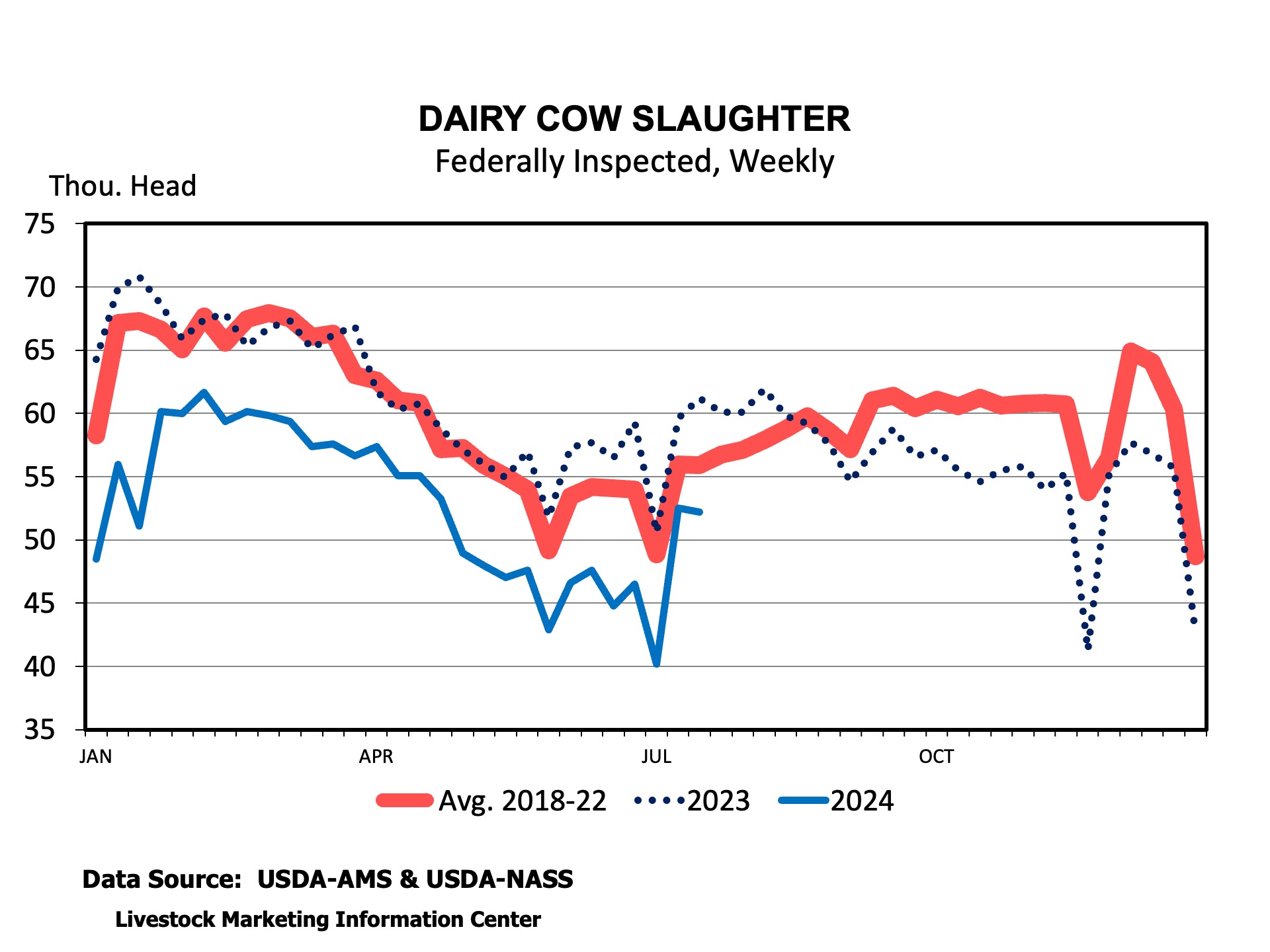
Dairy cow slaughter rebounded sharply in the two weeks after the holiday shortened fourth of July week. It’s pretty normal for dairy cow slaughter to climb seasonally after early July but, the magnitude of this weekly increase is larger than usual. Even with the rebound in culling, weekly slaughter remained smaller than last year and the average of the last 5 years. The trend of smaller dairy cow culling is likely to continue the rest of the year, even though culling may increase seasonally.
Over the last 8 weeks dairy cow culling is 18 percent smaller compared to the same time period last year. Dairy cow slaughter is reported by region. Region 4 (Southeastern states), region 6 (Texas, Arkansas, and Louisiana), and region 3 (Virginia and Pennsylvania) include Southern states. Dairy cow slaughter in regions 3 and 4 are down 10 percent and 8 percent, respectively. Slaughter in region 6 is down 32 percent. Regional differences in slaughter rates continue to indicate shifts in regional milk production with faster than average culling rates in the South but slower culling in the Southern Plains. On an interesting note, region 8, which includes Colorado and the Dakotas, has reported larger dairy cow slaughter this year than last year and is the only region to do so. Dairy cow culling is likely to remain relatively low in coming months due to fewer dairy cows in total, relatively few replacement heifers, and rising milk prices.
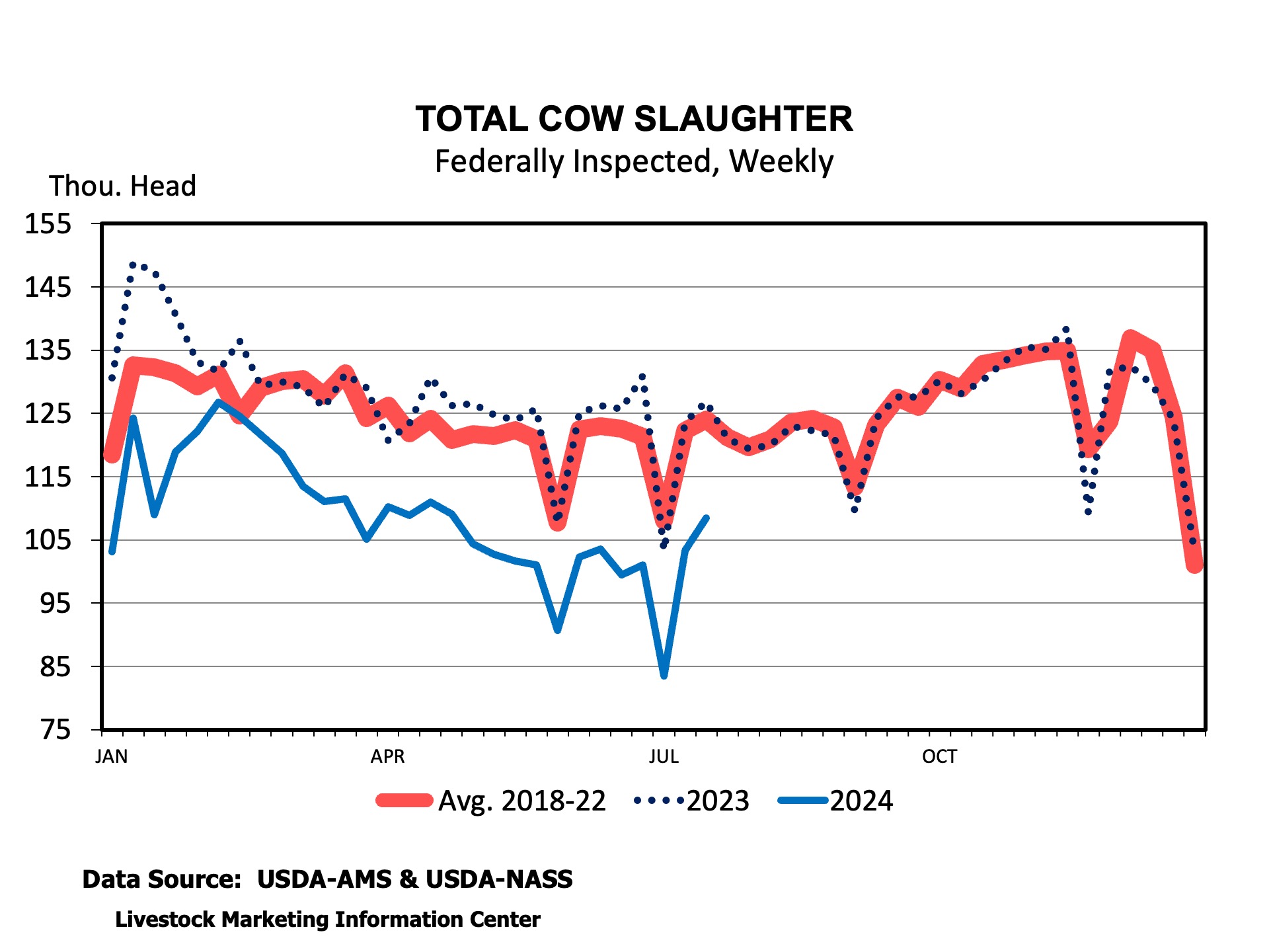
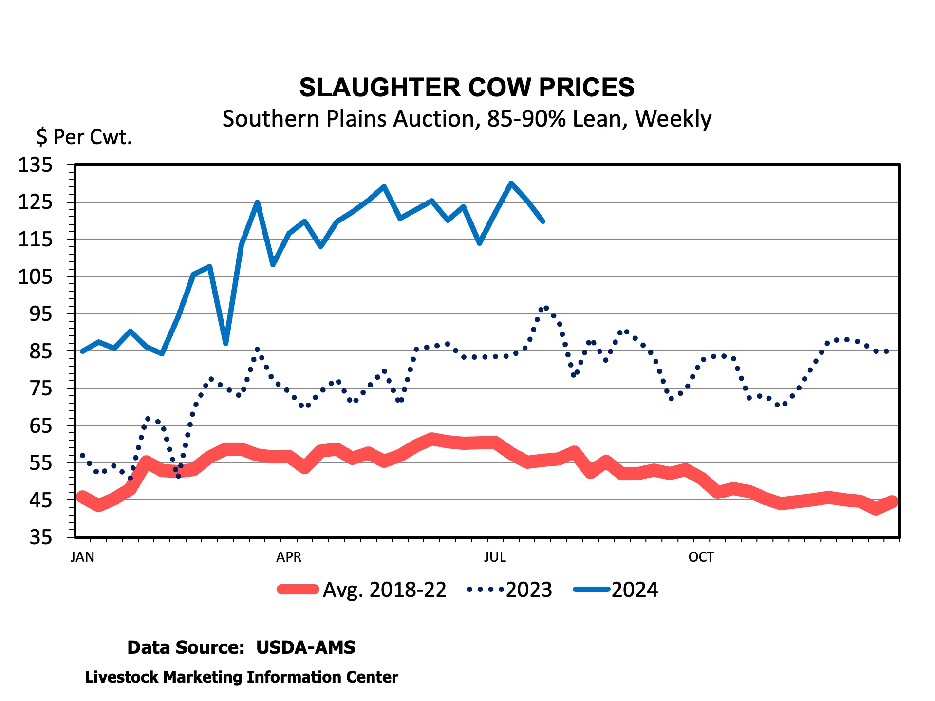
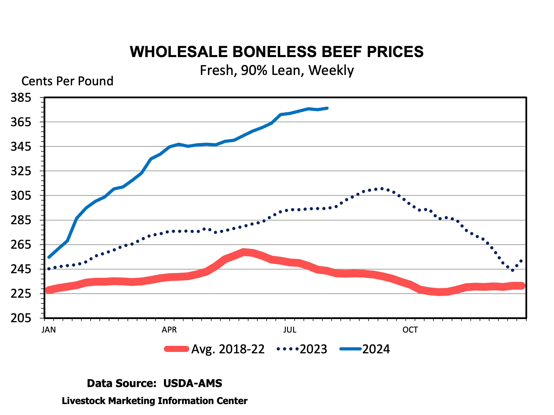
The overall decline in dairy cow slaughter is further supporting cull cow prices across the South and the country. Dairy cow slaughter has made up, on average, about 48.6 percent of all cow slaughter over the last decade. This year dairy cow slaughter represents 48.3 percent of all cow slaughter. Reduced dairy cow culling coinciding with reduced beef cow slaughter is further cutting supplies of lean beef. Wholesale boneless 90 percent lean beef hit a new high of $3.76 per pound last week. The cow-beef cutout is in record territory at over $290 per cwt. Lean slaughter cows at auction continue to hover around $125 per cwt. The lack of dairy replacements and need for replacements by some has bred dairy cow and heifer prices up from $300 to $600 per head in Kentucky dairy auctions.
Overall, reduced dairy cow culling is supporting cull cow prices. Reduced total cow culling is putting additional strain on cow packing plants across the region.
Gross Domestic Product (GDP) is likely the most closely watched and commonly cited economic indicator. GDP is “…the market value of all goods and services produced within a country in a given period of time” and is “…the best single measure of a society’s economic well-being” (Mankiw, 2007). While tracking and forecasting GDP is important for businesses, labor, investors, policymakers, and economists, it has important implications for the farm economy as well. GDP can be thought of as how well off your customers are to buy the things you produce.
The International Monetary Fund uses GDP to track global economic growth by country and country groups. Real GDP growth (adjusted for inflation) has exhibited interesting trends since 1980 that have implications for grain markets (Figure 1). From 1980 to 2000, there was very little difference between growth rates of GDP between advanced economies (e.g., U.S., Japan, most of Europe, Canada, Australia, U.K), and emerging market and developing economies (e.g., Brazil, Russia, India, China, Mexico). Advanced economies grew at an average rate of 2.9%, with emerging market and developing economies growing by 3.5%.
Figure 1. Global Economic Growth, real GDP, 1980-2029
In the early 2000s, world economic growth rates began to be driven by emerging economies. Gains in productivity, rising per capita incomes, and a growing middle class have made many emerging economies more competitive as suppliers to world export markets and increased the size of their domestic markets (Kose and Prassad, 2010). From 2000 to 2019, the growth rate of advanced economies was 1.9%, with emerging and developing economies growing by an average of 5.5%.
Since 2020, economic growth rates in emerging economies have slowed. Global conflicts, trade tensions, inflation, and rising interest rates are a few of the factors cited for a slowdown in economic growth, factors that hit emerging and developing economies especially hard (IMF, 2024). Estimates for 2020-2024 show advanced economies growing by an average of 1.5% and emerging and developing economies by 3.6%. Including forecasts by the IMF for the next five years, average GDP growth from 2020-2029 is projected to be 1.7% for advanced economies and 3.8% for emerging and developing.
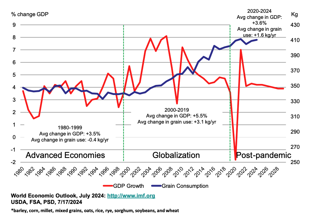
Figure 2. Real GDP growth in emerging and developing economies and world per capita grain consumption
Trends in world grain consumption have shown significant changes since 1980 as well (Figure 2; blue line). In 1980, consumption of barley, corn, millet, mixed grains, oats, rice, rye, sorghum, soybeans, and wheat was 348 kg per person. By the end of the 1999/2000 marketing year, that number was down to 340 kg. Then, per capita consumption began to grow, reaching over 400 kg by 2019. With increasing protein in diets and grain for fuel, the most recent estimate of world per capita grain consumption in 2024 is 410 kg.
An overlay of GDP growth in emerging and developing economies and world per capita grain consumption shows the relationship between these factors (Figure 2). From 1980-1999, a period with little difference between growth in advance economies and emerging economies, GDP grew by 3.5% while grain use per capita fell by 7 kg (-0.4 kg/yr). From 2000-2019, an era of globalization and expanding economic impact in emerging economies with GDP on the rise, grain use increased by 62 kg (+3.1 kg/yr). Since 2019, post-pandemic, with slower rates of growth in GDP, grain use has increased by 8 kg (1.6 kg/yr), about half the rate of growth of the previous 20 years.
Per capita grain consumption is one measure of global grain demand. Even if per capita consumption is unchanged, growth in the population base would still mean an increase in grain consumption. In 1980, the world population was increasing by 1.6% per year. In 2000, population growth was 1.3%. That growth rate is down to 0.9% in 2024 and forecast to be 0.8% by 2030, half the rate of growth in 1980 (USDA, ERS, 2024).
Important to levels of grain use are patterns of global economic growth, especially GDP growth in emerging and developing economies. As growth rates in this region slow down over the next decade, per capita grain use may yet increase, but at a slowing rate.
The combination of slowing population growth and a slowdown in economic growth may alter recent patterns in world grain use. That means gains in productivity (weather permitting) have a higher likelihood of exceeding gains in use. When that happens, that is a recipe for lower prices.
References:
International Monetary Fund (IMF). World Economic Outlook, July 2024, http://www.imf.org.
Kose, M.A. and E. Prassad. “Emerging Markets Come of Age”, Finance and Development, Vol. 47, No 4, December 2010.
Mankiw, Gregory. Brief Principles of Macroeconomics, Fourth Edition, Thompson South-Western, Mason, Ohio, 2007.