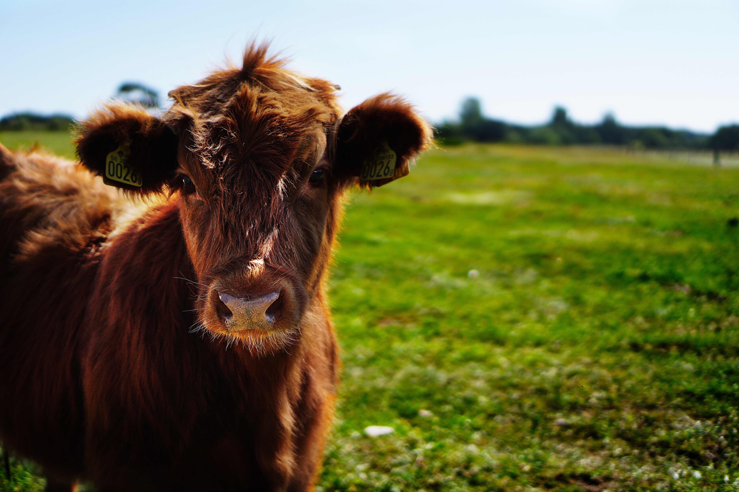
To breed or to feed, that is the question? In an October 2022 article, bred heifer values for 2023 were discussed. The projected value for bred heifers in Tennessee during 2023 was between $2,400 and $2,600, which is exactly the value that many of the bred heifers traded for in the spring. The question now is if a producer should retain heifers from the spring calf crop for breeding or if they should set wheels under them for feeding.
Despite bred heifer values hitting the price projection this spring for fall calving females, it is beneficial to consider the expected value for those animals moving forward. Given the expectation that calf values will hold firm, the bred heifer value could reach $3,000 to $3,200 per head this fall and moving into late winter. Thus, should a producer retain those animals and breed them, or should the producer sell the female at weaning or as a yearling? A weanling 550 pound heifer in Tennessee is currently valued near $1,265 per head while a load of 750 pound black heifers is valued near $1,770 per head (Figure 1).
The answer to this question is not simple. Here are a few considerations. First, are the heifers being retained and bred to go back in the retaining producer’s herd or are they meant for resale? If they are meant for the retaining producer’s herd then calf price projections moving forward are important. If the females are meant to be sold then a producer needs to make sure they have a marketing outlet for those females. Second, it takes feed, capital, and labor resources to retain heifers. If any of these are in short supply then critical pencil and paper work need to be done. Third, is it worth the risk to forgo the calf or feeder cattle value to breed females?
In closing, the demand for bred heifers or bred females, in general, is regional at this point. Some regions do not have the hay and forage resources to begin retaining heifers while other regions do. Producers should consider their resources and expected demand for bred females before jumping into this market.
Figure 1. Weekly Tennessee prices for 500-550 pound and 750-800 pound heifers.
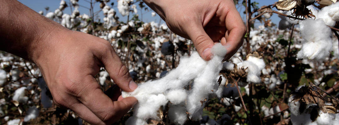
U.S. cotton is historically in relatively poorer shape this year. According to the USDA Crop Progress report, only 41% of cotton acreage is rated to be in good or excellent condition as of the first week of August, which ranks 5th worst over the past twenty years. This is driven by Texas – the largest producing cotton state – which has 55% of its acreage in poor or very poor condition. Therefore, it is not a huge surprise that the USDA lowered its cotton production forecast this year. As of the August Crop Production report, U.S. average upland cotton yield for 2023 is projected at just 773 lb. per acre, which if realized would be the fourth lowest yield in the last twenty years. The USDA also forecasts 8.5 million upland cotton acres to be harvested, which would suggest the abandonment rate – or percentage of planted acres that go unharvested – to equal 22%. Let’s look into the accuracy of the USDA’s August cotton acreage and yield forecasts in recent years to further understand where cotton production might end up.
Figure: Final Cotton Yield and Abandonment Rate with August Forecast Errors by Year
a) Final Cotton Yield and August Forecast Error
Data source: USDA-NASS Crop Production Note: Forecast error = Final Yield minus August Yield Forecast
b) Final Abandonment Rate and August Forecast Error
Data source: USDA-NASS Crop Production Note: Forecast error = Final Yield minus August Yield Forecast
Where is cotton production likely to end up? The above figure (panel a) shows annual ending cotton yield and the difference between the final yield and the August forecast, or the August forecast error. Cotton yields have been within 10% of the August prediction in fourteen of the past nineteen years, averaging a miss of just 2%. On average, cotton yield has ended up 20.9 lb. per acre higher than what was forecast in August. Abandonment was more difficult to predict, with the average year seeing the abandonment rate two percentage points higher than forecast in August, an 11% miss (panel b). Abandonment rates ended up higher than predicted in fifteen out of nineteen years, meaning that harvested acreage wound up lower than forecast.
Now what can history tell us about where production might end up in 2023? Let’s consider some low- and high-production scenarios from the previous nineteen years. Consider storm-plagued 2020 as a low-production year, which forecast 929 lb. per acre yields and a 24% abandonment rate in August but wound up with 841 lb. per acre and a 33% abandonment rate. As a result, production fell over 3 million bales short of what was forecast. An identical error to 2020 would result in yields 11% lower and an abandonment rate 6 percentage points higher, resulting in 11.0 million bales of production in 2023 (see table below). On the other hand, two years (2005 and 2022) both saw one-percentage point decreases in the abandonment rate and 11% increases in yield over what was forecast, and 2 million bales of unexpected production. A similar scenario this year would result in 15.4 million bales of production. This large range in potential outcomes could lead to additions or reductions to the forecast 2.99 million bale ending stocks, ultimately affecting the 79 cent per lb. marketing year price forecast. However, it is important to note that cotton use would likely be adjusted downward primarily through exports in a low-production scenario which would prevent cotton stocks from cratering.
Table 2: 2023/24 Cotton Production Scenarios Given Recent Forecast History
What happened to all the Black Farmers? As the 2023 Farm Bill approaches, this question has been asked a lot, and it should be since Black farmers have declined by more than 96 percent since 1920, with there being 926,000 Black-operated farms in that very year.
In order to understand why this has happened, the first step may be analyzing how exactly Black farmers finance their farm operations. This question is imperative when determining why there has been a drastic decline in Black farmers. To understand how Black farmers are funding their farm operations and the barriers to obtaining capital, the Policy Center set out to gather this information by bringing together 1890 Land-Grant Institutions in the nine states with the highest concentration of Black farmers to conduct in-depth research on these issues.
Each state participating in this project was asked to survey at least 100 Black farmers. The survey found that the top method for funding their farms was personal cash followed by ownership. This confirmed that Black farmers are not accessing loans to build their farm business. Access to capital for black farmers is a serious issue and the results showed that effective access to capital for black farmers is very limited. Consequently, black farmers applied for few loans and obtained a very low share of their operational capital from external sources.
There are many factors and complex interactions that add to this issue. Some levels of discrimination existed, as mentioned by some farmers in their response, but the fundamental causes of the issue go far beyond just discrimination. USDA has created new programming and initiatives but has not included actions to assist the Black farmer in catching up to farmers who have always received help, have a complete understanding, and thrive.
Things, such as a simplification of the application process, reduction of the down payment/credit needed, and help with the application process and getting farm numbers could increase the number of farmers applying for and receiving funding are things that can create changes for Black farmers, but there are clear systemic changes that needs to take place as well.
To access the full study, contact Dr. Kara Woods, research analyst at the Socially Disadvantaged Farmers and Ranchers Policy Research Center at Alcorn State University, at kawoods@alcorn.edu.
The planting phase of the crop production cycle comes with many risks. The amount of time available for planting is significant in determining whether all the fields intended for planting can actually be planted. For crops insured under the Federal Crop Insurance Program (FCIP), the final planting date, a component of the prevented planting provision of the FCIP, establishes the tail end of the planting window and helps to determine the amount of time available for planting crops each year.
Final planting dates vary by crop and location. The dates are chosen to increase the likelihood that insured crops achieve their highest attainable yields each year for a given county and crop. After the final planting date passes, farmers with crop insurance must decide whether to proceed with planting their intended crop or make a prevented planting claim.[1]Prevented planting claims have been known to vary significantly across states. How the final planting dates may influence those differences has not been thoroughly investigated. Generally, final planting dates are set earlier in the calendar year moving from north to south, reflecting the growing seasons that increase in length as one moves further south in the United States. For example, the final planting date for corn is May 31st in Kossuth County, Iowa; May 31st in Thomas County, Kansas; April 25th in Lonoke County, Arkansas; and April 15th in Evangeline Parish, Louisiana.
Differences in seasonal weather patterns, though, may affect the effective length of time available to plant as final planting dates change across states. Early spring rains and other weather variables (like temperature) can shorten or lengthen the planting window each year. To account for these differences, we can estimate the effective planting window between the first day available for planting and the final planting date by combing the USDA NASS estimate of days suitable for fieldwork with the final planting date. Here we construct the variable by using the first suitable day for planting according to the NASS estimate and calculate the average number of days suitable for fieldwork that occurs between that date and the final planting date for a county and crop. We use the average for the period 2011-2020 for corn for this example.
Figure 1a shows how the average effective planting windows change across states using corn as our example. Indiana, where the final planting date for each county is June 5th has, on average, roughly 29 suitable days for planting corn. Louisiana, having the earliest final planting date of April 15th of the states sampled, has the fifth greatest average number of days suitable for planting at roughly 25 days. A clear consequence of a shorter effective planting window is the effect it has on prevented planting claims. Figure 1b shows the percent of insured corn acres with a prevented planting claim for the period 2011-2020. In Figure 1a, the states are ordered by increasing effective planting window.
In general, both panels of Figure 1 together show that the prevalence of prevented planting acres runs roughly counter to the effective planting window prior to RMA’s final planting date. The exception, though, seems to be the Midwest states (Iowa, Illinois, and Indiana in this example) where the effective planting window appears to play no significant role at all, suggesting that other factors may be fundamental differences worth exploring in the Midwest states. Factors such as larger farm sizes and greater crop diversity in many southern states, for example, or a higher degree of tiled acres in the Midwest states, potentially play roles, likely compounding the effect of the shorter planting windows on the share of prevented planting acres relative to the Midwest.
Nevertheless, the final planting date paired with the NASS days suitable for planting appears highly correlated with the differences in prevented planting acres across states. The significance here is that final planting dates have been designed to consider total potential yield at harvest; however, the cost side of this cost benefit equation may include the risk of prevented planting claims during the planting period. Optimal final planting dates may consider both outcomes in determining optimal final planting dates.
Figure 1: a) Average number of suitable days for planting corn for 9 states across the Midwest and Southern United States. b) Average share of county acres with prevented planting claims.
Notes: Averages for 2011 – 2020. Average days suitable for fieldwork calculated as the sum of “Days Suitable for Fieldwork” as determined by USDA NASS between the first day suitable for fieldwork and the RMA final planting date. Sources: USDA NASS (2023), RMA Summary of Business (2023).
[1] More information on the decisions farmers face for planting occurring after the final planting date can be found here: Connor (2022); Biram and Connor (2023)
Determining the appropriate bid price for beef cows is important for buyers and sellers in the ranching industry. The Bid Price for Beef Cows decision aid is a practical and valuable tool that simplifies the bid price calculation and enables insightful “what if” analysis based on your financial expectations and productivity projections. This tool employs a net present value (NPV) approach, factoring in the desired return or discount rate.
Several variables play a significant role in determining the bid price for a cow, including: the total debt of your operation, operating costs per cow, estimated future calf prices, cull cow prices, required loan amount, interest rate, number of calves per cow, weaning weight, weaning rate, and more. In this example, we focused on the effect of higher interest rates in the bid process.
The amount of debt required for cow purchases and the interest rates directly affect the bid price. The higher the debt and interest rates, the lower the amount a buyer can afford to pay. For instance, an interest rate of 11% will reduce the bid price by $367 per head (Graph 1) compared to the 6% interest rate we may have seen a couple of years ago.
Figure 1: Beef Cow Bid Prices vs Interest Rates
In conjunction with operating costs, future calf prices are crucial in determining the bid price. Calf prices have increased in recent years as well as operating expenses. For the example bid prices in Fig.1, we assume an initial increase in calf prices for the next three years, followed by a slight decline. We expect prices to decline when the US cow inventory grows and US beef production increases. We also included a variable discount rate that rose to 7% with higher interest rate scenarios.
Using the Bid Price for Beef Cows tool will allow ranchers to analyze different scenarios and understand how much they should pay to restock their operations. Find the tool here (https://agecoext.tamu.edu/resources/decisionaids/beef/ ) and give it a try. Estimating reasonable future prices for your cattle and operating costs is imperative to better assess how much you can afford to pay for a replacement cow. By carefully considering these variables, you can make informed decisions and ensure the financial viability of your operation.