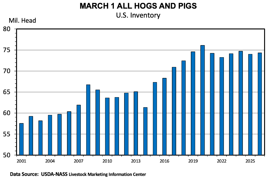
The latest USDA Quarterly Hogs and Pigs Report was released at the end of March and showed limited growth in the U.S. hog sector. Total inventory increased by 0.4 percent to just over 74.3 million head. This was within the range of pre-report expectations, but below the average pre-report estimates. Market hog inventories were also slightly higher, up 0.6 percent to 68.4 million head.
The more notable shift occurred in the breeding herd, which declined 1.5 percent year-over-year to just under 5.9 million head. This was below pre-report expectations, and the decline suggests producers remain hesitant to expand aggressively. In addition, USDA revised the December 2025 inventory, which reinforced the signal of limited expansion.
Farrowings during the December 2025 to February 2026 quarter were also lower than expected and declined 1.5 percent. This was the opposite of average pre-report expectations for modest growth. Productivity gains helped offset reduced farrowings. Pigs per litter increased 2.1 percent to 11.9. This was stronger-than-expected and pushed the pig crop up 0.6 percent to 33.2 million head.
Looking ahead, farrowing intentions signal producers are being cautious with production changes. Producers plan a slight increase in farrowings for March to May (up 0.1 percent) but a decline for June to August (down 2.1 percent). Supplies are expected to remain adequate in the near term but tighten later in the year, which could provide some support to prices.
Authors: Cesar L. Escalante, Joshua Emmanuel, and Naimul Bhuiyan
On October 2, 2025, the U.S. Department of Labor (DOL) issued an Interim Final Rule (IFR) that introduced several modifications in the determination of adverse effect wage rates (AEWRs) applicable to H-2A workers hired by U.S. farmers. The new methodology departs from relying on wage data from the Farm Labor Survey (FLS) and will instead set new AEWRs from wage information collected under the Occupational Employment and Wage Statistics (OEWS) survey of the Bureau of Labor Statistics.
This article pursues the arguments presented in our previous SAT article, which shows discrepancies in domestic-H-2A wage differentials at the national level due to the more aggregated nature of the old AEWRs. The previous BLS-based AEWR setting mechanism was riddled with the aggregation issues pertaining to geography, commodity and job type, and static annual AEWR levels.
The new AEWR setting scheme that H-2A employers are using this year resolves some of these aggregation issues. Specifically, state-level AEWRs are now set using the OEWS survey data, thus resolving issues associated with regional aggregation under the old system. In addition, there will now be two wage tiers for H-2A workers established according to the workers’ skill levels.
Level 1 – Entry Level AEWRs apply to positions with neither formal education nor specialized training requirements; and
Level 2 – Experienced Level AEWRs are set at higher rates “commensurate” to the skills, education, training, and/or experience requirements for such positions.
Finally, an adverse compensation adjustment (downward) is also available for employers that provide housing for their H-2A workers. The adjustment rate is determined as the “equivalent hourly rate based on the weighted statewide average of Fair Market Rents for a four-bedroom housing unit available from the Department of Housing and Urban Development.” (Congressional Research Service, 2025)
The new AEWR methodology’s intention to address wage aggregation issues is noteworthy. However, analysts and industry experts only acknowledge its partial resolution of the old system’s imperfections. Issues concerning how the OEWS survey is conducted and addressing job and commodity wage differentiation still exist. The wage data used in the survey comes from state unemployment insurance (UI) records. Because most farms are not included in those records, the survey mainly captures farm labor contractors and businesses that support agriculture rather than farms themselves. This can bias the results toward states with more labor contractors and may leave out states where farms are exempt from UI reporting.
While the new two-tier wage system is based on skill level, it is still calculated by averaging wages across several different farm job types. This means wages for crop workers, livestock workers, and equipment operators are combined into one state average, even though those jobs typically pay different rates. In practice, crop and nursery workers, who make up most H-2A employees, are usually paid less than livestock workers and equipment operators. Because their wages are averaged together, the AEWR can end up higher than typical crop worker pay. Some argue that setting a separate AEWR specifically for crop and nursery workers would better reflect actual farm labor markets.
All told, the recent changes in the AEWR setting policy are crucial, but merely intermediate steps in aligning AEWRs to wage market equilibrium conditions. Meanwhile, the DOL must continue to evaluate the need for further reforms that scrutinize and consider possible business and economic repercussions of unresolved “wage aggregation” areas in the AEWR determination scheme.
Table 1. Mean Wages for Selected Standard Occupation Classification (SOC) Codes and Adverse Effect Wage Rates (AEWRs), By Farm Labor Region, Fiscal Year 2024
Authors:Kodjo Barnor, Doctoral Student, Texas A&M University & Chrystol Thomas, Assistant Professor & Extension Specialist, Texas A&M AgriLife Extension
Data centers are moving into rural areas across the United States, hence competing with farmers and communities for land, water, and energy. Understanding what these facilities require and what they don’t offer in return is essential for rural communities. The key question is whether data centers complement or compete with agricultural operations. The answer depends largely on where they are located and how they use electricity, water, and land resources.
These facilities underpin artificial intelligence, cloud computing, and online services. Development is expanding rapidly across the United States, with Virginia and Texas becoming the most attractive locations due to their competitive electricity markets, abundant land, and growing renewable energy capacity (Figure 1). Texas has roughly 4 gigawatts (GW) of capacity, with almost 8 GW under construction, and could surpass Virginia as the largest global data center market by 2030 [1].
Figure 1. 2025 year-end leased data center and hyper-owned capacity (GW).
Note: From North America data center report year-end 2025, by A. Batson, 2026, Jones Lang LaSalle (JLL). https://www.jll.com/en-us/insights/market-dynamics/north-america-data-centers
What Kind of Facilities Are We Talking About?
Data centers vary widely in size. Small edge facilities serve local networks, while hyperscale facilities built by companies such as Amazon, Google, and Microsoft can span hundreds of acres and consume as much electricity as a small city (Table 1). These large facilities are increasingly locating in rural areas where land is available, and energy infrastructure can be expanded.
Table 1: Major Data Center Types and Typical Characteristics
Type
Typical Size
Power Demand
Land
Water Use
Hyperscale
100,000+ sq ft
100+ MW
100–1,000+ acres
Up to several million gal/day
Cloud
50,000–200,000 sq ft
10–99 MW
10–40+ acres
Moderate to high
Enterprise
10,000–50,000 sq ft
1–10 MW
5–15 acres
Thousands gal/day
Edge/Micro
<10,000 sq ft
<1 MW
<1 acre
Minimal
Notes: Source: Northeast Regional Center for Rural Development (NERCRD). 2026. Definitions are approximate and may vary by project design, location, technology, and operational requirements [2].
Energy Use
Unlike agricultural electricity use, which is seasonal, data centers operate continuously. A 100 MW facility running around the clock consumes roughly 2,400 megawatt-hours of electricity per day which is comparable to the daily electricity use of tens of thousands of households. In Texas, ERCOT forecasts that peak electricity demand could reach 218 gigawatts by 2031, compared with a record peak of 87 gigawatts in 2025 [3]. Data centers are expected to contribute significantly to this growth.
For irrigators and other large electricity users, rising demand could mean higher electricity rates and greater grid stress during summer months when agricultural demand peaks. Large industrial loads may also require transmission upgrades, and rural electric cooperatives could face infrastructure costs that ultimately affect rates for agricultural customers.
Water Use
Many data centers rely on evaporative or hybrid cooling systems requiring significant water withdrawals. A facility using one million gallons per day consumes more than 1,100 acre-feet annually; a hyperscale campus can require several times that amount. In regions overlying the Ogallala Aquifer, the Trinity, the Carrizo-Wilcox, or other stressed groundwater systems, this additional demand is not trivial.
Texas groundwater law follows the rule of capture, meaning landowners generally have the right to pump groundwater beneath their property unless regulated by local groundwater conservation districts. A data center developer purchasing land in your area has the legal right to withdraw substantial groundwater without compensating neighboring agricultural operations, unless local limits are in place. Producers should engage their local groundwater conservation district early in any proposed development process to understand what protections exist.
Land Use
Data centers compete with agricultural land uses on a long-term basis. Once developed, these sites rarely return to agricultural production. This is a tradeoff that deserves careful evaluation in communities where farmland values underpin local economies. While projects can generate property tax revenue and construction employment, they typically employ relatively few workers once operational. A large facility may require only a few dozen full-time employees. Also, some developers are pairing data centers with nearby solar or wind generation to meet sustainability targets and stabilize energy costs. These projects may create opportunities for landowners.
Conclusion
Data centers are becoming an increasingly visible feature of rural America. While they can generate local revenue, they also place continuous demands on electricity and groundwater resources used by agriculture. Communities considering these developments should evaluate key issues in advance: which aquifer will supply water and at what volumes, whether transmission upgrades are required and who will bear the costs, the long-term employment footprint, and whether the overall economic benefits outweigh potential pressures on local infrastructure and resources. Careful evaluation of these factors will help communities better manage the expansion of data infrastructure across rural areas.
References
[1] Batson, A. 2026. North America data center report: Year-end 2025. Jones Lang LaSalle (JLL). https://www.jll.com/en-us/insights/market-dynamics/north-america-data-centers.
[2] Northeast Regional Center for Rural Development (NERCRD). 2026. Data Centers: Assisting Communities in Understanding the Challenges and Opportunities. Webinar presentation slides, February 24. Pennsylvania State University.
[3] ERCOT. 2025. Long-Term Load Forecast Report. Electric Reliability Council of Texas.
[4] Houston Advanced Research Center (HARC). 2026. Thirsty Data: Water Use and the Projected Data Center Boom in Texas.
The United States has a long and storied history of providing food aid to those who are in need around the world. One of the earliest examples dates to 1812 when the U.S. government sent $50,000 of wheat flour to Venezuela following a devastating earthquake. U.S. international food aid efforts were formalized with passage of the Food for Peace Act in 1954, which sought to alleviate global hunger while also disposing of domestic agricultural surpluses. In total, the U.S. has consistently spent in excess of $4 billion per year on international food aid and is, by far, the world’s largest contributor.[1] That funding results in more than 1 million metric tons of U.S.-grown agricultural commodities—including corn, sorghum, rice and wheat— being shipped to recipient countries each year, serving as a consistent source of demand and helping to stabilize domestic prices.
Over the last 200 years, policymakers have regularly debated the appropriate role of the U.S. government in providing international food aid. For example, during Congressional debates in 1847 about whether to send aid in response to the Irish Potato Famine, President Polk threatened a veto, arguing that it was his “solemn conviction…that Congress possesses no power to use public money for any such purpose.” For decades, policymakers have also debated the appropriate balance between food aid and development assistance—the proverbial “give a man a fish and you feed him for a day, teach a man to fish and you feed him for a lifetime.” Both featured prominently in the development and passage of the Food for Peace Act over 70 years ago, and both remain a prominent feature of American global food security efforts today.
More recently, the debates over international food aid have been more technical in nature, largely focused on the efficiency of food aid (or the perceived lack thereof) and the impact of that aid on the recipient country. On the latter, an amendment to the Food for Peace Act from Senator Henry Bellmon (R-OK) in the International Development and Food Assistance Act of 1977 required the U.S. government to assesses whether the recipient country has adequate storage facilities and whether assistance would interfere with the recipient country’s agricultural economy before shipping aid.
Despite these efforts, criticism of in-kind aid (i.e., U.S.-grown commodities) has resulted in a push for procurement of food aid in local/regional markets and for cash transfers for people to use in local shops. In 2010, the Obama Administration introduced a cash-based assistance program known as the Emergency Food Security Program (EFSP) that was designed to complement U.S.-grown commodities by allowing local/regional purchases along with cash transfers. Since then, the use of cash-based assistance has rapidly expanded, now accounting for more than half of international food aid provided by the United States. This has led to growing concerns among policymakers about a lack of accountability with cash-based assistance and the ease with which it can be misappropriated in recipient countries.
This brings us to Spring 2025. As part of their efforts to improve government efficiency and ensure U.S. international efforts are yielding promised results, the Trump Administration eliminated the U.S. Agency for International Development which oversaw Food for Peace, absorbing those efforts into the broader State Department. In December 2025, USDA entered into an interagency agreement to take over the administration of Food for Peace. In March 2026, the Committee on Agriculture in the U.S. House of Representatives marked up its farm bill proposal—the Farm, Food, and National Security Act of 2026—which would permanently transfer the authorities of the Food for Peace Act from USAID to USDA while reserving 50% of Food for Peace resources for U.S. grown commodities, returning the program “to its original intent of addressing the global hunger crisis through the purchase of U.S. grown commodities.”[2]
For many in the agricultural community, the shift to local/regional procurement and cash-based food assistance—however well intentioned—was undermining the historic mission of Food for Peace. Moving Food for Peace to USDA presents an opportunity to refocus the program, helping ensure that it can survive another 70 years in fulfilling its dual mission of using domestic agricultural surplus to help feed those in need around the world.
The USDA released the 2026 Prospective Plantings Report on March 31. Nationally, producers intend to plant fewer corn acres and more soybeans and cotton. Corn acreage is projected at 95.3 million acres, down 3.5 percent from the 2025 actual planted acreage, while soybean acreage is expected to increase 4.3 percent to 84.7 million acres. Cotton acreage is also forecast higher, up 3.8 percent to 9.64 million acres. These shifts reflect relative price signals and input cost considerations that have increasingly favored soybeans and cotton over corn in many areas.
In the Southern region, prospective plantings generally follow national trends, though the magnitude varies across states. Texas, the largest corn producing state in the South, is projected to increase acreage by 4 percent to 2.6 million acres. Kentucky, the second largest corn state in the region, is projected to reduce acreage by 4.6 percent, to 1.45 million acres. Meanwhile, the third largest corn state in the region, Tennessee, is projected to increase acreage by 7.5 percent, to 1.0 million acres. Mississippi is projected to see the largest decline, down 31 percent to 630 thousand acres, followed by Arkansas, down 27 percent to 590 thousand acres.
For soybeans, the Southern region is projected to increase planted acreage by 10 percent, led by Arkansas and Mississippi. Arkansas is projected to plant 3.1 million acres, up 19.7 percent from last year, while Mississippi is expected at 2.3 million acres, up 27.1 percent. Kentucky, North Carolina, and Tennessee round out the top five soybean states in the region, with acreage changes of 2.8 percent, 4.3 percent, and no change, respectively.
For cotton, the Southern region is projected to increase planted acreage by 4 percent to 8.94 million acres. Texas continues to dominate regional production, with acreage rising 3.7 percent to 5.52 million acres. Several states are projected to see notable gains, including Louisiana, up 22.2 percent, Tennessee, up 22 percent, North Carolina, up 19.3 percent, Oklahoma, up 15.4 percent, and Georgia, up 7.8 percent. In contrast, acreage declines are expected in Arkansas, Mississippi, and Virginia, down 9.6 percent, 9.1 percent, and 4.1 percent respectively. Meanwhile Alabama and South Carolina are projected to see no change.
For rice, the Southern region is projected to see a sharp reduction in planted acreage, declining 21 percent to 1.64 million acres. Arkansas remains the largest rice producing state, though acreage is projected to fall 22 percent to 1.0 million acres. Mississippi shows the largest percentage decline, down 51 percent to 80 thousand acres. Louisiana and Texas are also projected to reduce acreage by 10.8 percent and 13.8 percent, respectively. Overall, the decline reflects weaker market signals and continued input cost pressure across the region.
A large reduction is also expected in peanut acres, with the Southern region projected to reduce planted acreage by 14.4 percent to 1.65 million acres. Georgia remains the dominant producer, though acreage is projected to decline 15.2 percent to 780 thousand acres. All but Alabama are expected to see reductions, with Arkansas, South Carolina, and Texas all down more than 20 percent, and Mississippi, down 43 percent. Smaller declines are expected in Florida, North Carolina, Oklahoma, and Virginia. Alabama peanut acres are expected to increase 2.6 percent.
It is important to remember that this report reflects prospective plantings rather than final acreage. These estimates are based on producer surveys conducted in early March and are subject to change. A number of factors could influence actual planted acreage moving forward. In particular, these estimates likely do not fully capture the potential impact of the Iran conflict on fertilizer prices and planting decisions. Weather also plays a critical role in determining how much acreage gets planted. For producers, these figures serve as an early benchmark of current expectations that can be used when evaluating how evolving market conditions and weather may shift final planted acreage.
Table 1. 2026 Prospective Planting Acreage in the Southern Region (thousand acres)
Note: Acres are reported in thousand acres. Percent change represents 2026 intended plantings relative to 2025 actual planted acres. Dashes indicate negligible or unreported acreage. Source: USDA Prospective Planting Report, March 31, 2026.