Southern wheat producers are experiencing significant losses this year due to low prices, weather conditions, and a shortage of stockers for grazing. To maximize returns or minimize losses, farmers must evaluate whether producing wheat for grain, grazing, or hay is most financially viable under current market and production conditions.
We have a Wheat and Small Grains Decision Aid (Link) to help farmers decide whether to use wheat for grain, grazing, or baling. To make an informed choice, compare the prices of grazing, wheat hay, and grain, expected yields, production costs, crop rotation options, available equipment, and insurance coverage. What follows is an example analysis with basic assumptions, check out the decision aid to include your operation-specific data.
Although all alternatives show negative returns this year, hay production continues to offer higher profits under similar conditions. In this example, baling hay is more favorable due to lower wheat grain prices. Actual results will depend on your wheat bale prices and may vary if you own harvesting or baling equipment.
Grazing is also more favorable if farmers were able to graze wheat early, have sufficient moisture and forage, and enough livestock to maximize beef production.
The decision aid enables you to compare alternatives from both economic and financial perspectives. Analyzing cash flow helps identify the most advantageous option, particularly if you own a combine or hay baling equipment.
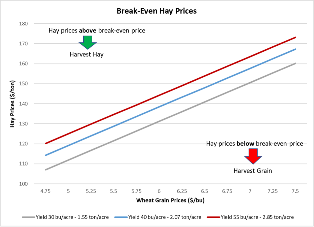
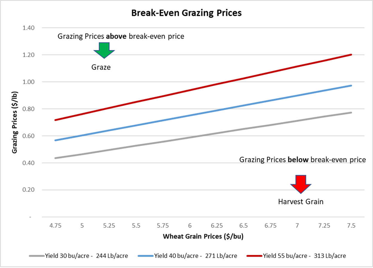
You can also use this information to determine the hay sale price needed to match wheat grain profit margins or to set an appropriate grazing price. The Decision Aid uses your data and costs to calculate breakeven prices for hay and grazing (see Graphs 1 and 2).
Graph1: Break-Even Hay Prices
Consider baling wheat if you can sell hay above the breakeven price, based on current wheat prices and expected yields. For example, with a yield of 40 bushels per acre at $5 per bushel, baling is preferable only if the net price per ton of hay exceeds $119, assuming 76% of the estimated biomass or 2.07 tons per acre.
Graph 2. Breakeven Grazing Prices
Similarly, with a yield of 40 bushels per acre at $5 per bushel, grazing is advisable only if the grazing price exceeds $0.60 per pound of gain.
With low wheat prices, alternatives such as grazing or hay production may provide better financial outcomes. The Wheat and Small Grain Decision Aid (Link) is designed to help farmers evaluate these options. Using your own data on yields, prices, and costs is essential for effective analysis. If you need assistance with the decision aid, please let us know.
Consumers are interested in native plants (i.e., those present prior to European settlement) with heightened demand in recent years. Interestingly, positive perceptions of native plants are widespread but spending in the U.S. is uneven, with heightened spending among a relatively small group of consumers. Using a 2022 national survey of 2,066 U.S. households that purchase plants, consumer spending patterns reveal a clear segmentation story relative to native plant purchasing behavior. Consumers can be divided into three segments based on their perceptions of native plants: Native averse (32% of the sample), native curious (36%), and native enthusiast (32%). Approximately 20% of the sample (n=422) were from the USDA South region (i.e., Delaware, Washington D.C., Florida, Georgia, Maryland, North Carolina, South Carolina, Virginia, West Virginia, Alabama, Kentucky, Missouri, Tennessee, Arkansas, Louisiana, Oklahoma, Texas; USDA, 2021). Of the Southern participants, 25% were native averse, 42% were native curious, and 32% were native enthusiasts.
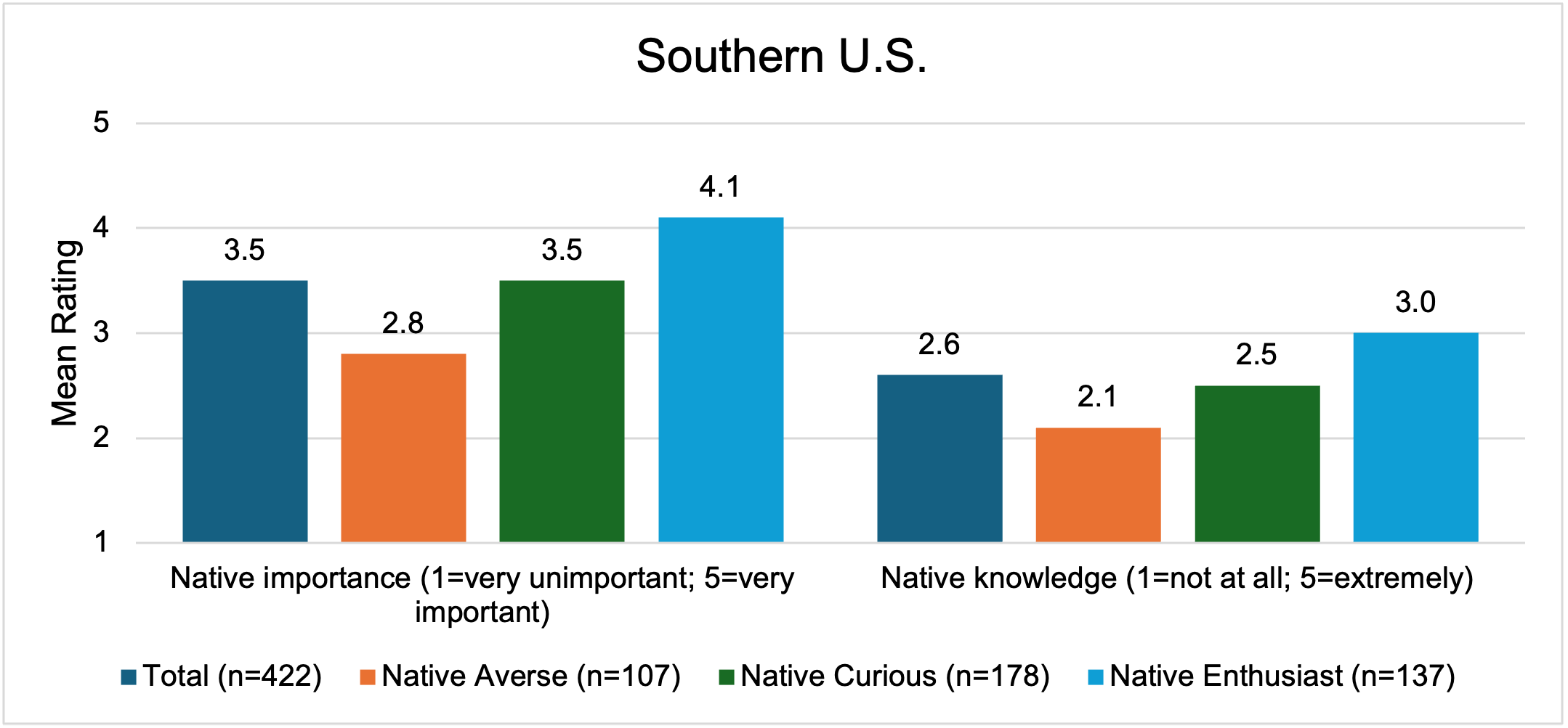
Several factors influenced segment membership including native plant perceptions, education, and plant purchasing behavior. Native enthusiasts and native curious consumers perceived native plants as providing many benefits (i.e., less maintenance, adapted to difficult sites, help water conservation, benefit the economy, improve biodiversity, are readily available, I know where to purchase native plants, are drought resistant, help pollinators, complements existing landscape, aid in natural habitat restoration, are aesthetically pleasing, and wildlife friendly) while native averse consumers did not share these perceptions. Rather, the native averse segment perceived native plants as not providing significant benefits over introduced species. The native enthusiasts also placed greater importance on native plants (in general) and reported higher subjective knowledge (Fig. 1). Similar results were observed in the U.S. and Southern region. In the South, 100% of native enthusiast members purchased native plants in 2021 (similar to 100% in the U.S. total sample), vs. 45% of native curious (46% in the U.S. total sample), and 34% of native averse segments (28% in the U.S. total sample). Education impacted segment membership, with native enthusiasts and native curious having higher education levels than the native averse group. Income did not influence segment membership, indicating that disposable income was not the driving factor behind these groupings, rather perceptions influenced subsequent plant spending behavior.
Figure 1. U.S. Consumers Perceived Importance and Knowledge of Native Plants
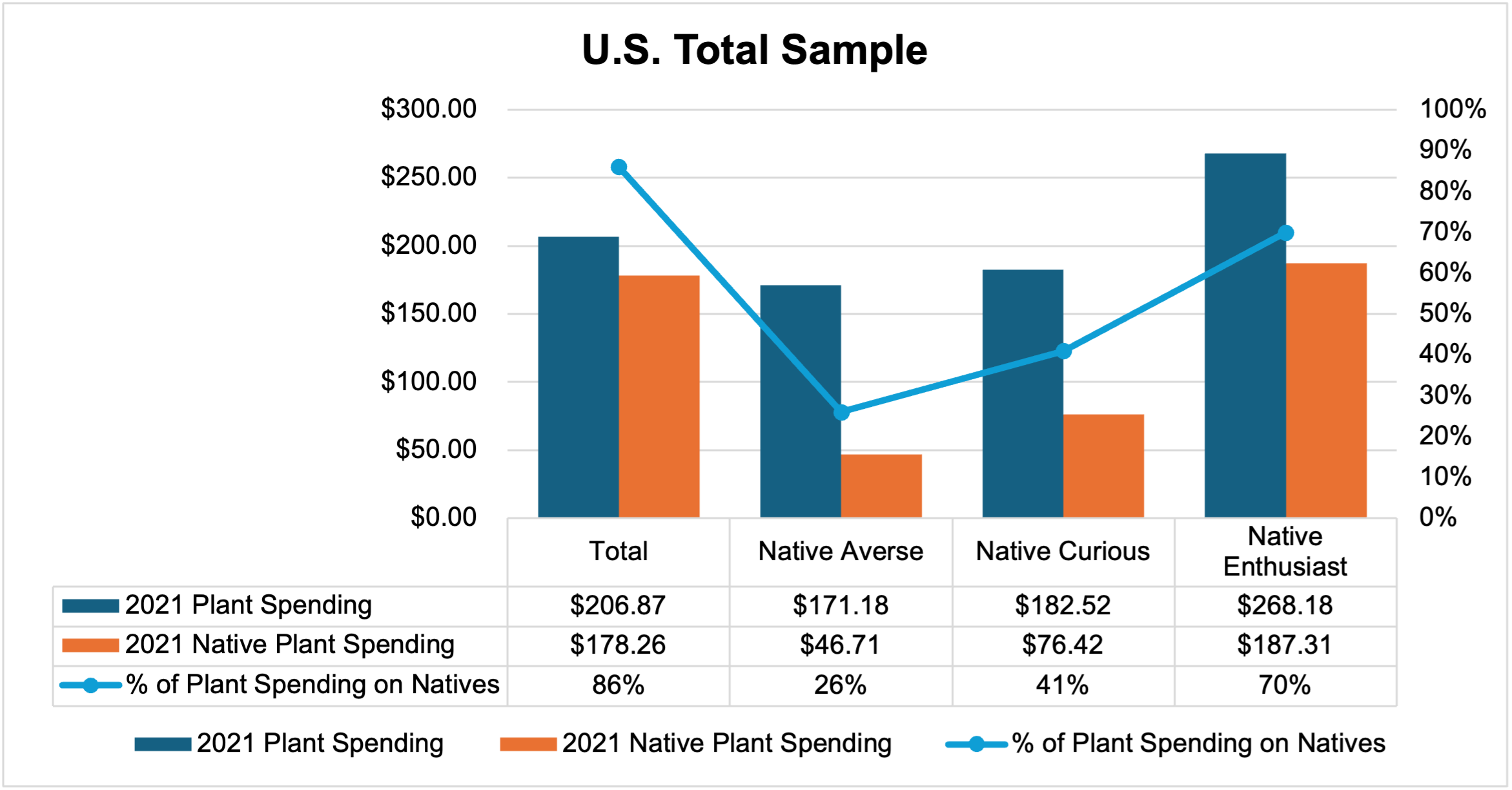
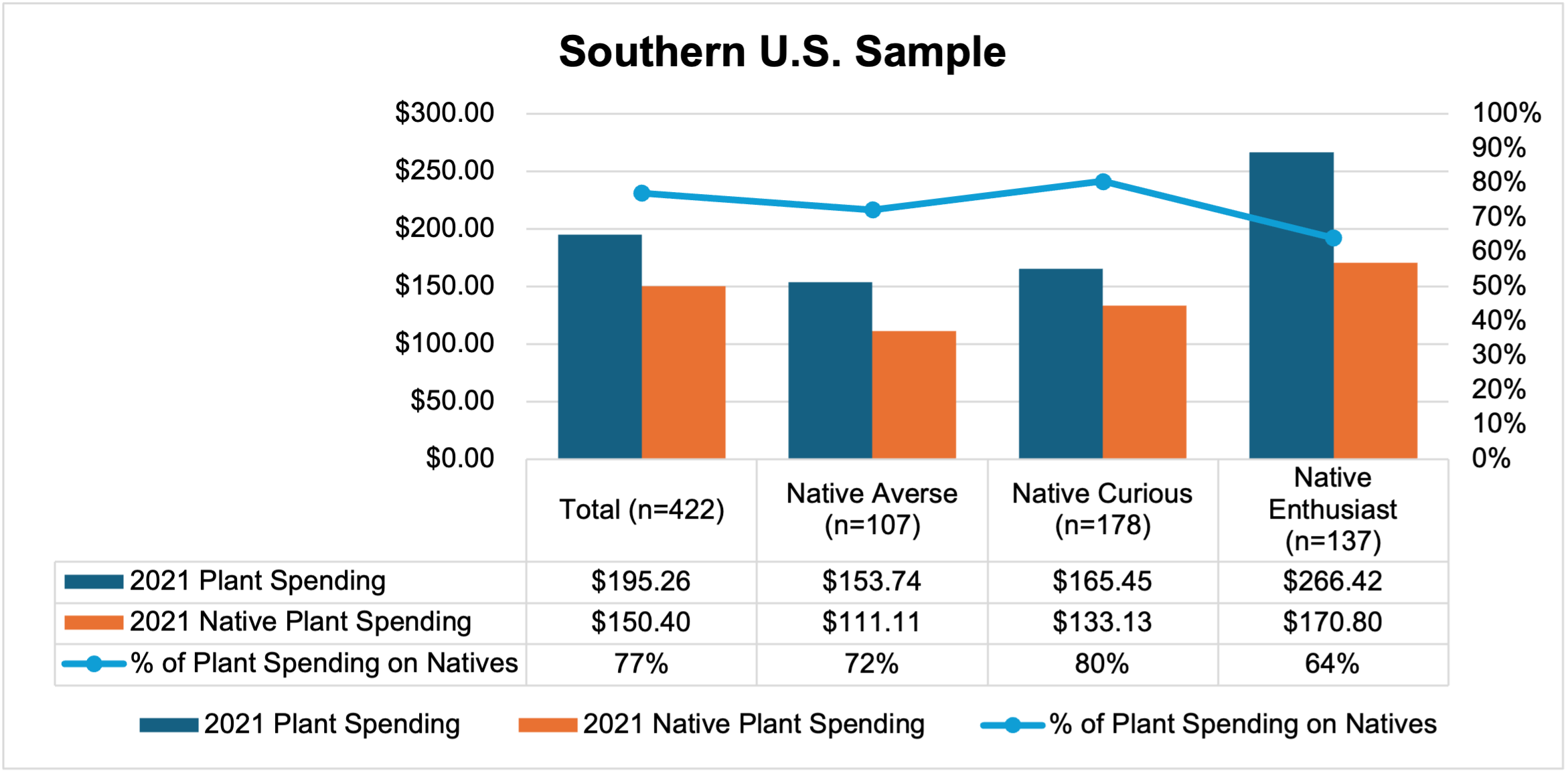
While all three segments purchase native and introduced plants, native plant expenditures are primarily driven by native enthusiasts and native curious members (Fig. 2). On average, in 2021, native enthusiasts spent $187 on native plants (70% of total plant spending), while native curious consumers spent $76 (41% of total plant spending) on native plants, and native averse spent $47 (26% of total plant spending) on native plants. In 2021 in the Southern region, native enthusiasts spent $171 on native plants (64% of total plant spending), while native curious consumers spent $133 on native plants (80% of total plant spending), and native averse spent $111 on native plants (72% of total plant spending). Of note, total plant spending was higher among native enthusiasts in both the total and Southern samples relative to the native curious and native averse which were not significantly different. This implies that the native enthusiast segment is spending more on plants in general and are likely seeking out native plants when they are available.
Figure 2. U.S. Consumer Native and Introduced Plant Spending Behavior In 2021 (n=2066).
These patterns point to potential growth in native plant sales through increasing per-customer spending among consumers who already buy plants and view native plants favorably. A small shift in the native curious consumers’ plant budgets to purchase more native plants could generate a sizable gain in total native plant sales because of the size of the segment and their receptiveness to native plants. For growers, retailers and landscapers, strategies that increase confidence in native plant selection is key. For example, clear labeling, aesthetic assortments and bundling native plants with information may be more effective than broad awareness campaigns. These strategies may be more impactful given that there is evidence that native plants are not always clearly identified at retail (Brzuszek and Harkess, 2009) and that native plants may be perceived as less desirable than introduced plants (Gillis and Swim, 2020). Thus, providing clear point-of-sale information about the plants and their benefits while demonstrating their aesthetic appeal may aid in convincing members of the native curious segment to purchase more native plants.
References:
Brzuszek RF, Harkess RL. 2009. Green industry survey of native plant marketing in the southeastern United States. HortTechnology 19:168-172. https://doi.org/10.21273/HORTTECH.19.1.168
Gillis AJ, Swim JK. 2020. Adding native plants to home landscapes: The roles of attitudes, social norms, and situational strengths. J Environ Psych. 72: 101519. https://doi.org/10.1016/j.jenvp.2020.101519
Acknowledgements: This research was supported by a grant from the Horticultural Research Institute (‘‘HRI’’). Its contents are solely the responsibility of the authors and do not necessarily represent the views of HRI.
Source: Rihn, A.L., A. Torres, B. Behe, and S. Barton. 2024. Unwrapping the native plant black box: Consumer perceptions and segments for target marketing strategies. HortTechnology. 34(3): 361-371. https://doi.org/10.21273/HORTTECH05401-24.
While farmers have been dealing with inflation in input costs since the onset of COVID-19, relatively high commodity prices (in large measure resulting from the war in Ukraine) helped blunt the pain through 2022. The perfect storm arrived as commodity prices started plummeting in 2023. Over the last 3 years—from 2023 to 2025—the losses have been piling up. As noted in Table 1, the average corn, soybean, and wheat producer has accumulated roughly $300 per acre in total losses over the last 3 years. For cotton producers, that estimate is roughly $1,000 per acre. After all their crops have been sold and all their bills have been paid, that’s how far in the hole they remain. Thankfully, the federal government has stepped in at various times to help. But, this all begs the question of what the net result over the last 3 years has been. This is especially the case as calls continue to circulate on Capitol Hill about the need for additional bridge assistance.
As noted in Table 1, Agriculture Risk Coverage (ARC) and Price Loss Coverage (PLC) provided little assistance for 2023 and 2024 largely because the reference prices had not been updated since the 2018 Farm Bill. While ARC and PLC will deliver significantly more assistance for the 2025 crop year—owing to improvements in the One Big Beautiful Bill from last summer—that assistance is not slated to arrive until later this year (October 2026). Congress also stepped up in December 2024 and created the Emergency Commodity Assisstance Program (ECAP), providing $10 billion in assistance for economic losses incurred in the 2024 crop year. More recently, Secretary Rollins announced an additional $11 billion for row crop producers via the new Farmer Bridge Assistance (FBA) program for economic losses incurred in the 2025 crop year.
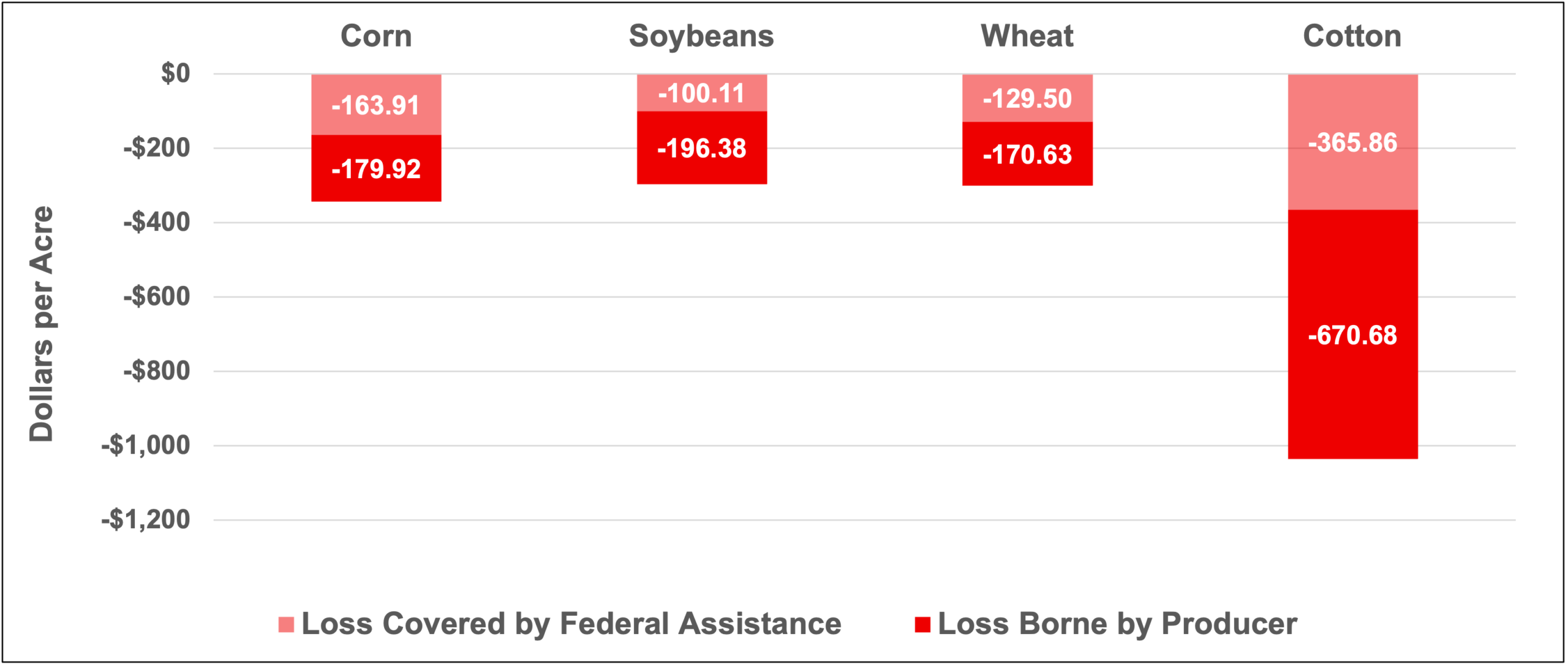
That is a tremendous amount of assistance. Is more really needed? While we will leave the question of “need” to policymakers to debate, we do offer the following observations. As reflected in Table 1 and Figure 1, despite all of the aid provided, we estimate that it is covering roughly 35% of the total loss for cotton and soybeans and roughly 45% of the loss for corn and wheat. In other words, farmers have had to shoulder roughly 55% to 65% of the loss on their own over the last 3 years. If nothing else, this should bring into focus the magnitude of the challenge they’ve been facing. Perhaps most daunting: they are facing a situation where the outlook suggests the losses will grow even larger next year.
Table 1. Cumulative Farm Losses for the Major Row Crops, 2023-2025F.
2023-2025F Cumulative Totals
Corn
Soybeans
Wheat
Cotton
Total Revenue ($/ac)
2,333.29
1,675.04
883.67
1,760.67
Total Cost ($/ac) a/
2,677.12
1,971.53
1,183.80
2,797.21
Net Returns ($/ac)
-343.83
-296.49
-300.13
-1,036.54
ARC/PLC ($/ac) – 2023-24 Crop Years
10.98
10.50
4.94
30.72
ARC/PLC ($/ac) – 2025 Crop Year b/
65.66
28.97
54.52
133.05
ECAP ($/ac) – 2024 Crop Year
42.91
29.76
30.69
84.74
FBA ($/ac) – 2025 Crop Year
44.36
30.88
39.35
117.35
Total Farm Bill & Ad Hoc Assistance ($/ac)
163.91
100.11
129.50
365.86
Share of Loss Covered by Aid
48%
34%
43%
35%
Figure 1. Share of Cumulative Farm Losses for the Major Row Crops Covered by Federal Assistance and Borne by Producers, 2023-2025F.
Now, for a couple of technical points. First, some may ask why we didn’t include crop insurance indemnities or natural disaster aid (think the Supplemental Disaster Relief Program) in our analysis. The reason: our total revenue estimates in Table 1 use marketing year average prices and harvested yields. Our assumption is that any crop insurance indemnities or disaster aid payments simply help partially restore producer revenue. As a result, total revenue is an appropriate proxy. Second, some may ask why we focused only on the 4 major row crops with more than 10 million base acres. The primary reasons for this were that the ARC/PLC average payments are very sensitive to acreage assumed, and there is a significant difference between base and planted acreage for these smaller-acreage crops. While that will likely change with the new addition of base acres in the One Big Beautiful Bill, it remains a limitation for analyzing the 2023-2025 period that would likely skew our results. Further, for some of the smaller-acreage crops, payment limits are significantly binding. Without a reliable way to incorporate the effects of payment limits into this analysis, the estimated payments would be significantly over-stated. While some of these challenges also impact the major row crops, in our opinion, they are less pronounced. So, while we may follow up on this analysis in the future, for today we focused on the 4 major row crops.
Bottom line: for the major row crops, while the federal government has provided a significant amount of assistance, farmers are shouldering even more of the loss, and they are facing a growing season in 2026 that may well compound the loss even more. In dealing with the uncovered losses already incurred, producers have only so many options: (1) watch their equity erode in proportion to the losses they’ve faced; (2) to the extent that equity is gone they can [try to] borrow money to cover the losses; or (3) they go out of business. They are going through that mental math while also trying to cash flow the upcoming year.
One final point: we appreciate more than most the difficulty of getting anything done in Washington, D.C. We also encounter producers every day who are very grateful that policymakers have stepped up to the plate to help keep them on their farms during these very trying times. But, we’d be remiss if we didn’t also note that over the last 3 years, as a nation, we’ve essentially been asking farmers to put their livelihoods on the line – with very little hope for profits – to keep raising food and fiber…while hoping that the federal government will deliver relief at the 11th hour to help keep them there. One of us is married to a rocket scientist…but it doesn’t take a rocket scientist to know this isn’t sustainable.
Commodity prices are influenced by a wide range of factors, but seasonal patterns remain an important consideration for crop marketing decisions. Even in periods of heightened volatility, understanding how prices tend to behave at different points in the marketing year can help producers evaluate timing risk and opportunity. Using soybeans as an example, this article examines historical price seasonality to illustrate how these recurring patterns can inform marketing strategies.
Seasonality reflects the tendency for prices to follow recurring patterns throughout the marketing year, largely driven by changes in supply availability. Across crops, prices are often weakest near harvest, when supplies are most abundant, and strengthen later in the year as stocks are drawn down. While this pattern is widely understood, it is not universal. In some years, crop prices are stronger at harvest than during the remainder of the marketing year; however, these “harvest-strong” years are relatively rare and tend to behave differently than the typical seasonal pattern.
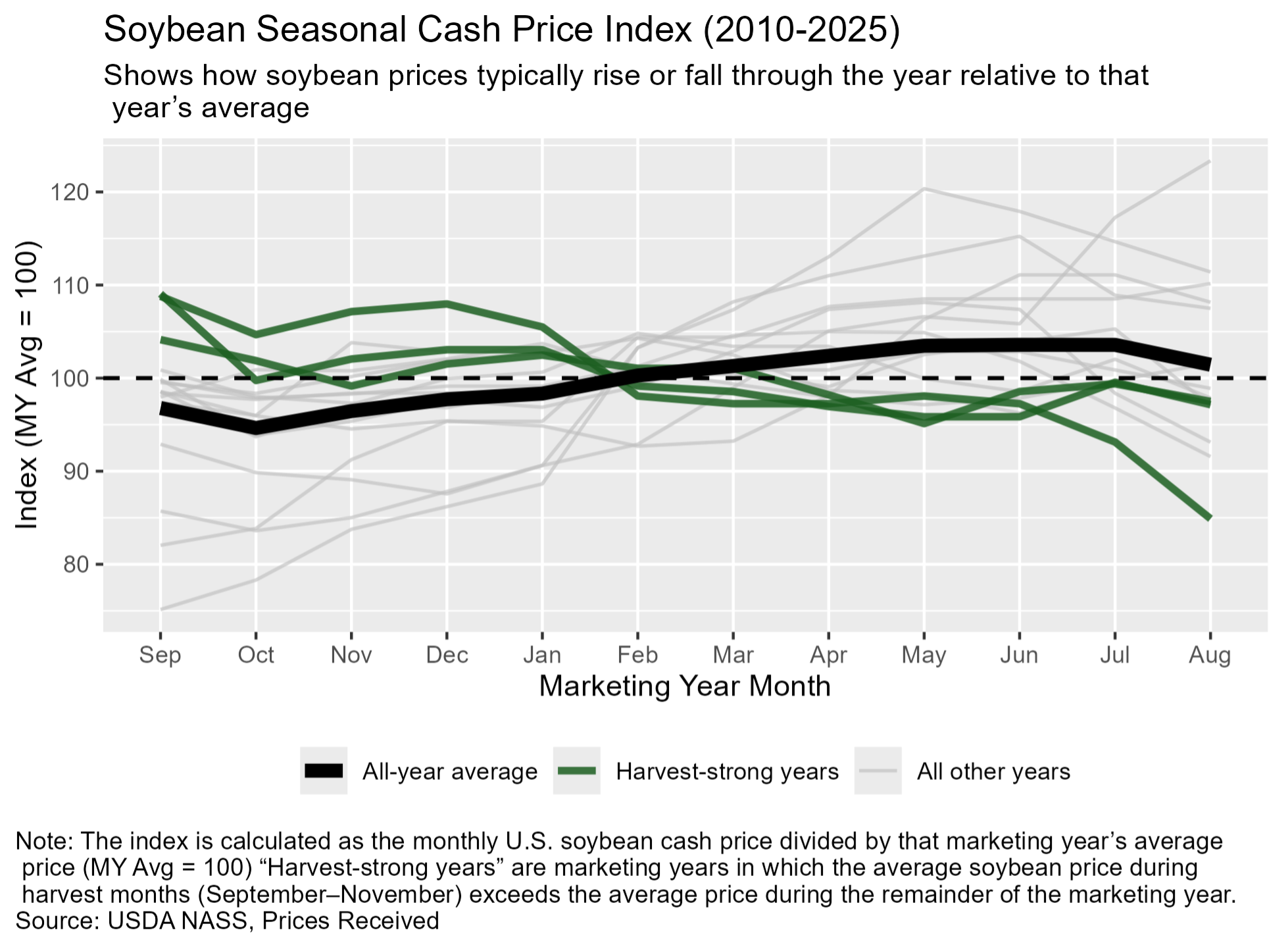
Figure 1 illustrates soybean cash price seasonality using national monthly prices from 2010–2025. Prices are expressed as an index, calculated by dividing each month’s price by that marketing year’s average price. A value of 100 represents the average price for the year, while values above (below) 100 indicate prices that were higher (lower) than average.
The thick black line in Figure 1 shows the average seasonal pattern across all years. This long-run average confirms a familiar story: soybean prices tend to be relatively weaker in the early fall, strengthen through winter and spring, and often peak in late spring or early summer before declining as new-crop supplies approach. From a seasonal perspective, this pattern suggests that pre-harvest and late-spring marketing opportunities often outperform harvest-time sales.
Not all years follow this average path. The green lines in Figure 1 highlight harvest-strong years—marketing years in which average soybean prices during harvest (September–November) were higher than prices during the remainder of the marketing year. The lighter gray lines represent all other years. Over the past 15 years, soybean prices were higher at harvest in only three years: 2015, 2019, and 2024. In 2015, harvest prices were supported by weather risk and relatively tight global balance sheets. In 2019, prices were influenced by trade uncertainty and a delayed supply response. Most recently, in 2024, tight stocks and global supply concerns helped support prices at harvest. In contrast, the remaining years exhibit stronger pricing opportunities outside the harvest window.
This distinction has practical marketing implications. In most years, weak harvest prices are followed by some degree of seasonal recovery, making post-harvest marketing opportunities more attractive. When prices are unusually strong at harvest, however, the historical record suggests that price upside later in the marketing year may be more limited.
The key takeaway is not that producers should market at the same time every year, but that seasonality provides a useful baseline expectation. When prices align with typical seasonal patterns, historical averages can help frame marketing decisions. When prices deviate, particularly when harvest prices are strong, it may signal that capturing favorable prices sooner deserves consideration. Incorporating seasonal patterns alongside market fundamentals, risk tolerance, and cash-flow needs can help producers make more disciplined and informed soybean marketing decisions.
USDA released the Cattle inventory survey on Friday, January 30th. We’ve included some thoughts on the report from a few of our Southern Ag Today Livestock Economists.
Kenny Burdine, University of Kentucky.
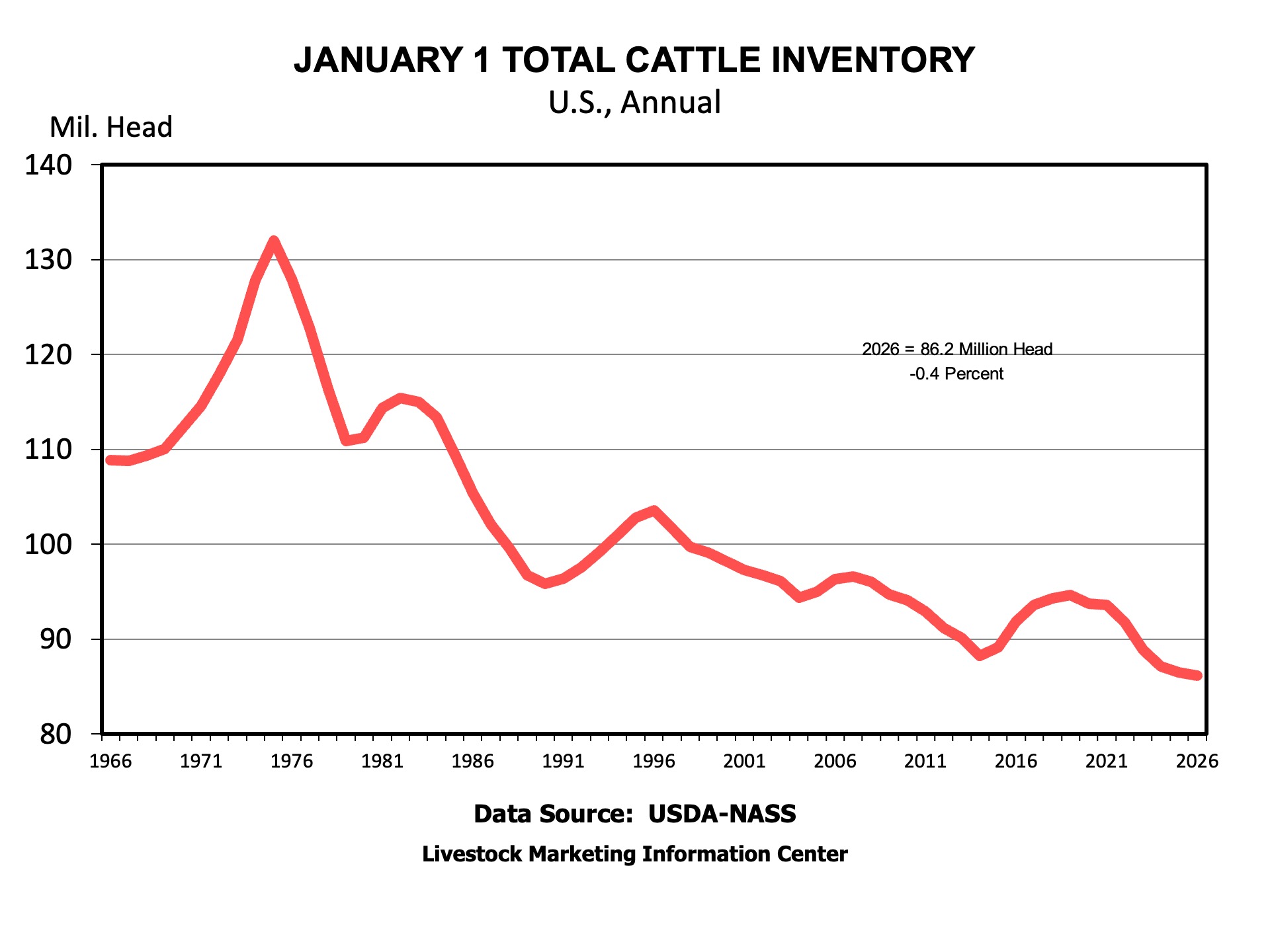
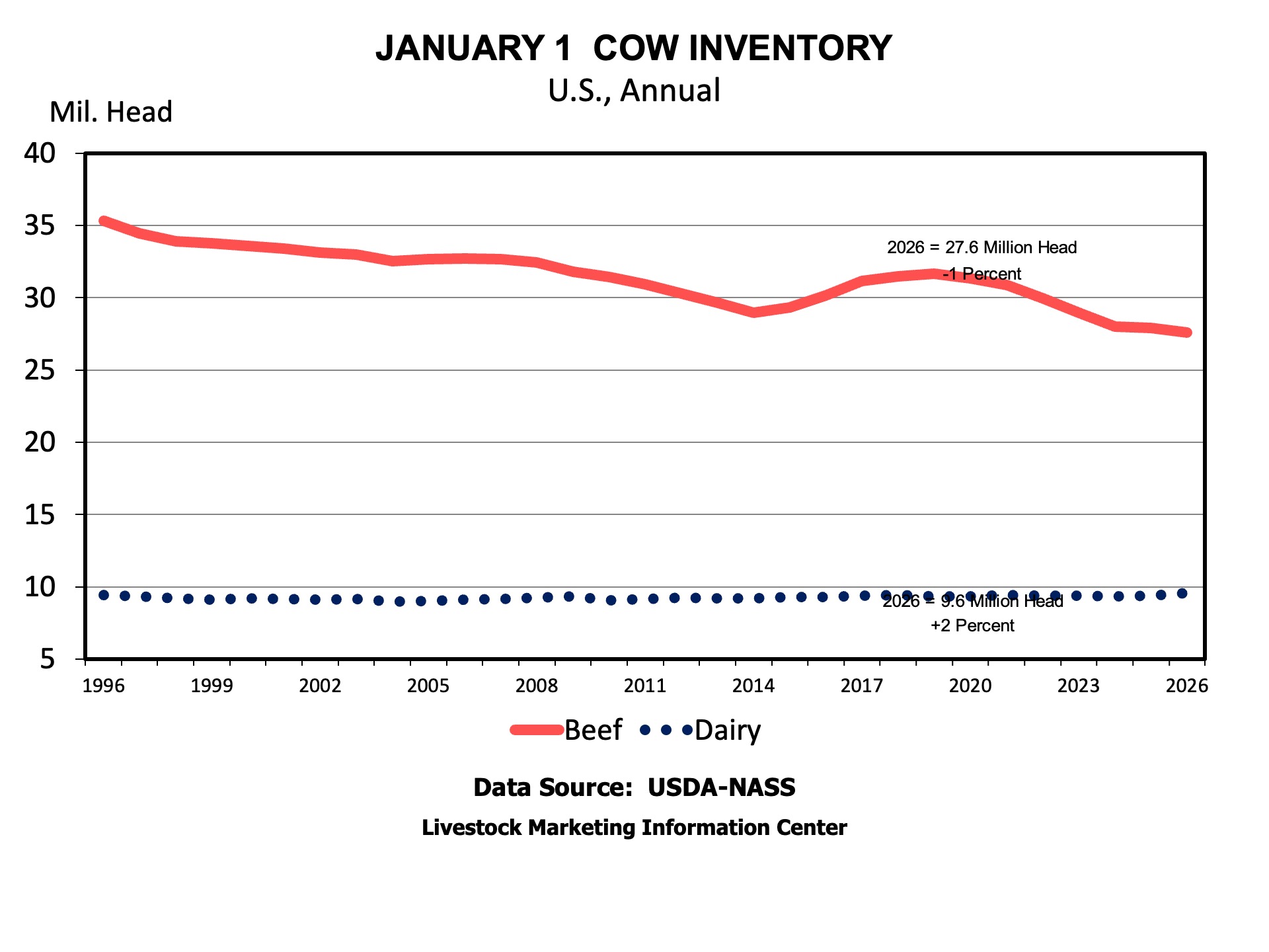
In a word – bullish! The 1% decrease in beef cow inventory surprised me. With beef cow slaughter down by over 500,000 head in 2025, I expected beef cow numbers to be up slightly coming into 2026. At 27.6 million cows, the US beef herd is still at its lowest level since 1961.
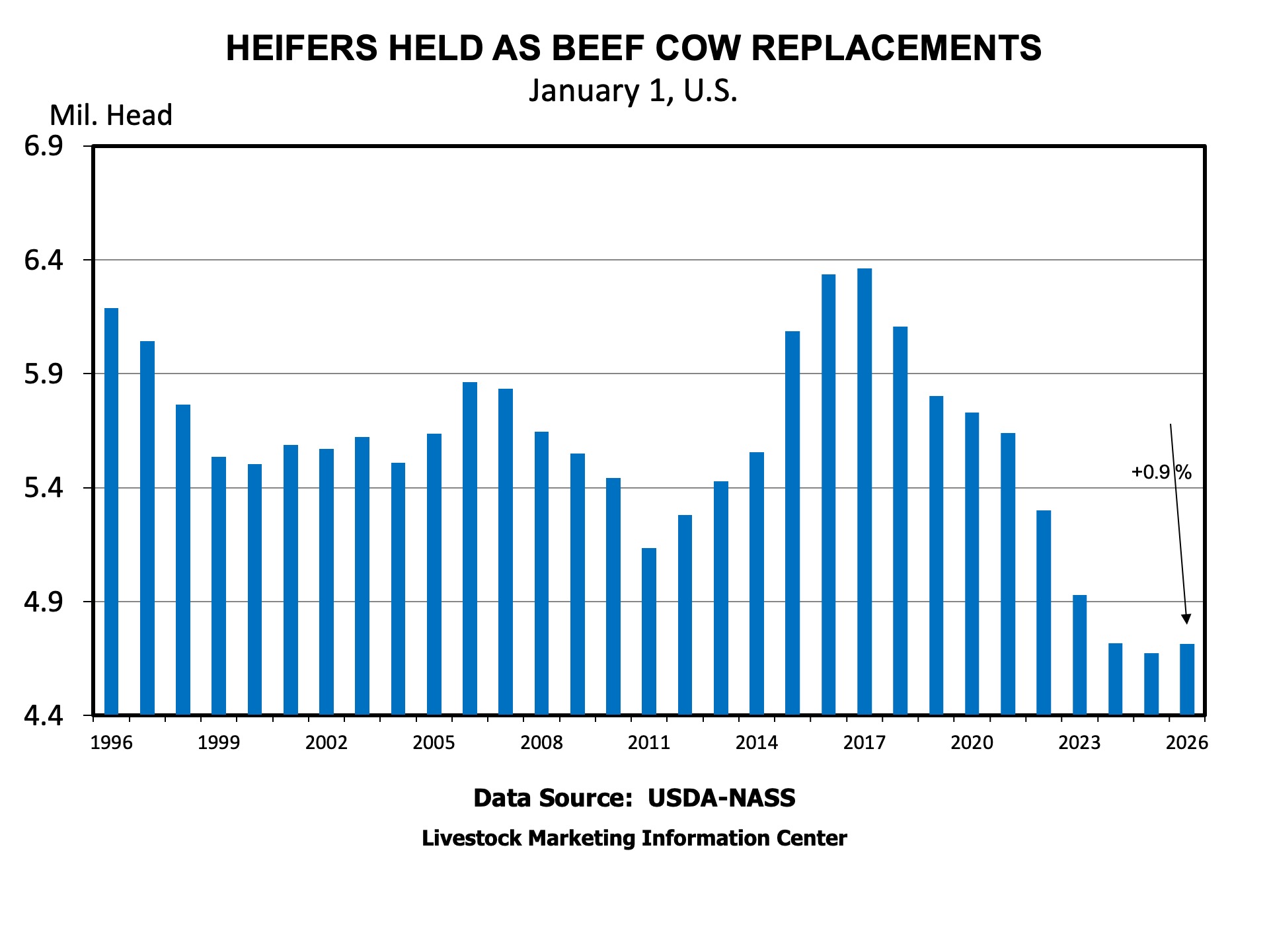
Heifers held for beef cow replacement were estimated at a little over 4.7 million head, which is up 0.9% from last year. I like to consider this number as a percent of beef cow inventory, which would be 17.1%. This is below the long run average, but higher than each of the last 3 January reports.
The 2% increase in dairy cow inventory is also noteworthy. 2024 was a very good year in the dairy sector and cow numbers seemed slow to respond. However, monthly estimates started rising steadily during 2025 and that was reflected in this January 1 number. While milk prices have fallen sharply over the last 12 months, that is likely being offset by strong values for beef-sired dairy calves.
KY beef cow inventory was estimated down another 7,000 (-0.8%) head this year. This is the lowest beef cow numbers have been in the Commonwealth since the 1960’s. In addition to production costs, female values (weaned heifers and cull cows), and interest rates, expansion of the Kentucky cowherd is further constrained by limited pasture availability. A lot of pasture ground was converted to row crops over the last couple of decades.
Andrew Griffith, University of Tennessee.
NASS January 1, 2026 cattle inventory did not perfectly align with industry expert expectations. Frankly, I thought industry experts were a little too ambitious with their numbers before the release of cattle inventory estimates. I am a little surprised more heifers were retained for beef cow replacement than a year ago, but then again, a year ago was a relatively low quantity of animals. As it relates to Tennessee, the values look in line with what was expected, which was a decline in beef cow numbers and heifers held for replacement. Three consecutive Falls have brought drought to Tennessee, which puts a damper on heifer retention.
Hannah Baker, University of Florida.
Some small revisions to the 2025 survey were noted. Revisions to the 2025 data reduced total cattle and calf inventory by 190,000 head, while beef cow numbers increased by 28,500 head. After these revisions, cattle and calf inventory declined by less than 1%, with beef cow numbers down 1% heading into 2026. In Florida however, total cattle inventory increased by 1.3% (20,000 head), with beef cow numbers up 7,000 head (0.8%) and dairy cow numbers up 3,000 head (3.1%). Following a 3,000-head increase in 2025, Florida beef producers appear to be moving toward herd stabilization. Heifers held for beef replacement remained unchanged at 115,000 head. Prolonged statewide drought conditions, recent freezing temperatures, and high calf prices will certainly influence decisions regarding more significant heifer retention in 2026.
Max Runge and Ken Kelley, Auburn University.
Total cattle and calves in Alabama increased slightly for a second consecutive year, even as portions of the state experienced drought. Beef cows that have calved were essentially unchanged from a year ago, while beef replacement heifer numbers increased modestly. At this point, these changes appear to reflect herd stability rather than clear evidence of expansion, and it remains too early to determine whether producers are beginning a broader rebuilding phase.
Will Secor, University of Georgia.
The USDA Cattle report’s headline all cattle and calves inventory was not totally surprising; it showed a slight reduction. However, digging into some of the details reveals interesting shifts. The most interesting national number to me was seeing that the number of beef replacement heifers increased. This is a sign that producers are starting to re-build or at least slow the pace of liquidation. For Georgia, all cattle and calves dropped by around one percent, largely driven by beef cow numbers dropping by around three percent. Milk cow numbers offset those beef cow declines partially, as these increased by five percent. Finally, Georgia’s 2025 calf crop rose by two percent compared to 2024. This higher calf crop came from fewer cows in 2025 compared to 2024 – a potential indication of improved reproductive efficiency for operations in the state.
David Anderson, Texas A&M.
Fewer beef cows but more beef cow replacements, up 50,000 head to 650,000, were noted in the Texas inventory data. Way in the back of the report was the annual estimate of the number of stocker cattle on small grain pastures (wheat, oats, etc.) in Texas, Oklahoma, and Kansas. The report indicated 180,000 more stockers, up 12 percent, than a year ago. That’s interesting given the drought that hurt pasture development, relatively few cattle available, and high prices.
Josh Maples, Mississippi State University.
This report sets up 2026 as another year of tight supplies and provides support for strong prices. The number of heifers held back for beef cow replacements was 4.714 million head, which is a 0.89 percent increase from a year ago. This was on the low end of pre-report estimates. This is the first annual increase in beef heifers in a decade, but still a very low total and not a clear signal of herd expansion. Perhaps this report is a sign of the herd stabilizing as we move into 2026, but more retention will be needed to suggest herd expansion. The bulk of the increased heifer retention occurred in Texas, which added 50,000 heifers for beef cow replacement, while the U.S. overall added 41,700. If more heifer retention occurs in 2026, it will be interesting to track the regional differences in where that growth happens. Total cattle and calves in Mississippi decreased one percent to 800,000 head.
Overall, fewer beef cows will keep supplies tight and prices high in the coming months and the next couple of years.