USDA NASS has released the equivalent of college football’s pre-season poll, which is the August Crop Production report (released August 12). The Crop Production report provides an estimate of acreage, area harvested, yields, and production for the major row crops in the U.S. Additional crop production reports (polls) will be released in September, October, and November. The Annual Crop Production report (final poll) will be released in January.
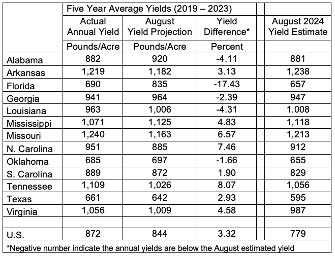
For the states represented in the Southern Ag Today area, estimates for cotton yields garner a lot of attention. How accurate are these August estimates to actual yields? Table 1 shows the actual five-year average (2019 – 2023) annual cotton yield compared to the five-year average of the August yield projection.
Table 1. Annual Cotton yield vs. August estimates yields (5-year averages)
There is a range in the percent difference in the actual yields versus the August estimates. The actual five-year average ranges from 17.43 percent below the five-year estimated August yield (Florida) to just over 8 percent higher than the August estimate (Tennessee).
Like pre-season polls, the estimated yields can vary from the actual annual yield for numerous reasons. Wind and excess rain from tropical weather events cause the largest decline in yields from the August estimate to the actual yields. While we won’t know for several months what our actual yields are (or our favorite team’s record), the pre-season projections provide some insight.
Cattle prices have reached record highs, and the cattle herd is the smallest since the 1950s. USDA predicts high domestic prices will result in increasing imports in the coming years. The U.S. is an attractive market, particularly for lean beef trimmings for ground beef. This article briefly discusses the recent spike in live animals, fresh/chilled, and frozen meat imports.
During the first half of 2024, imports of beef and live cattle soared. From January to June 2024, the U.S. imported 175,441 more head of cattle than in the same period last year, a 19% increase, reaching 1.12 million animals (Fig. 1). Over the same span, imported Fresh/Chilled and Frozen beef rose 11% and 29%, totaling 331,550 and 365,067 metric tons (MT), respectively (Fig. 1). Tight lean supplies along with high domestic beef prices help explain the growth in foreign acquisitions.
As the U.S. cattle herd declines, live animal imports have increased, mostly from Mexico (Fig. 2). Drought in Mexico and high U.S. cattle prices helped fueled more U.S. feeder cattle imports. In 2023, Mexican sales to the U.S. jumped 43%. That is 375,879 more head of cattle than in 2022. The Mexican herd has been stable recently, with FAS-PSD/USDA forecasting 0.4% growth in 2024.
Imported fresh or chilled beef has been growing over the past decade (Fig. 3). In 2023, the U.S. imported more than double the quantity it did in 2013 (Fig. 3). During this period, Canada provided, on average, half of the U.S. imported fresh/chilled meat while Mexico had, on average, 34% of market share. FAS-PSS/USDA predicts Canada stocks will drop 2% in 2024, down to 11.06 million head.
The amount of foreign frozen beef increased by 20% from 2022 to 2023, totaling 0.57 MMT last year (Fig. 3). In 2013, Australia and New Zealand each held 41% of the frozen imported beef market. However, their market shares declined to 28% and 29% over the last decade. A two-year drought (2019-20) affected Australia’s supply. Since 2020, shipments from Brazil expanded, reaching 90,303 MT in 2023, representing 16% of the market share. When China temporarily banned Brazilian beef imports in 2021, Brazil diverted its products to other countries, including the U.S. According to FAS-PSD/USDA, Brazil’s (-0.92%) and New Zealand’s (-1.66%) cattle herds are expected to decrease in 2024, while Australia’s stock is projected to increase by 4.93%.
U.S. beef imports are likely to continue ahead of last year as fewer cows are culled, and lean beef supplies continue to shrink. Drought in Mexico will be a major factor in feeder cattle imports in coming months.
Figure 1. The U.S. Total Imported of Live Animals, Fresh/Chilled and Frozen Beef, Quantity: Jan – Jun 2023 vs. Jan – Jun 2024.
Source: FAS-USDA (2024).
Figure 2. U.S. Live Cattle Imports from Canada and Mexico, 2013-2023.
Source: FAS-USDA (2024). Note: Total quantity imported of live cattle other than purebred or those imported (HS code: 1022940).
Figure 3. The U.S. Total Imported Fresh/Chilled and Frozen Beef, Quantity: 2013-2023
Source: FAS-USDA (2024).
References
FAS-PSD/USDA (2024). PSD Reports. Livestock and Poultry. Retrieved from: https://apps.fas.usda.gov/psdonline/app/index.html#/app/downloads
FAS-USDA (2024). Standard Query. Retrieved from: https://apps.fas.usda.gov/gats/ExpressQuery1.aspx
USDA’s June Grain Stocks report estimated 37% more corn and 44% more soybeans stored on-farm than last year (Maples, 2024). Many producers are still sitting on unpriced old crop corn trying to decide whether to sell or hold through harvest hoping for prices to improve. This article discusses three potential options for a farmer deciding what to do with old crop held in storage. The three options – using 100,000 bushels of corn and a current cash price of $4.00 – examined are:
sell corn at the current market price;
continue to store corn with operating loan utilization; or
store corn with cash resources.
Selling corn at the market price is the most straightforward option. Selling would result in collecting $400,000 that could be used in other areas of the operation – including paying down opertating debt or covering expenses – or it could be invested. Additionally, making sales would free up storage for the new crop and shift the focus to marketing the 2024 crop.
If an operating loan with a 9% interest rate is being used, continuing to store corn until February would incurr interest expense of $21,000 ($400,000 × 9% × 7/12). Dividing by 100,000 bushels, the per-bushel interest expense would be $0.21 or $0.03 per bushel per month, meaning cash prices from now until February would need to increase to at least $4.21 for the farmer to be better off than selling at today’s prices.
If the farmer is using cash reserves, rather than an operating loan, to carry corn until February, forgone interest should be estimated. Current certificate of deposit (CD) rates for short term money are close to 4.5%. Utilizing $400,000 cash has a forgone return on investment interest of $10,500 ($400,000 × 4.5% × 7/12) or $0.11/bu ($0.015 per bu per month).
When deciding to continue to store corn or sell, several factors need to be considered. Calculating the interest expense or forgone interest is one factor. There is uncertainty in price direction; however, based on current projections it is likely that both futures prices and basis will remain low as harvest proceeds. It is worth noting that this analysis only considers interest expenses. It does not include other other storage costs or risks, such as quality losses, grain handling, and capital recovery for storage infastructure. Additionally, prices may not increase by February, and all storage could result in a loss.
References
Maples, William E. “Having a Way Out.” Southern Ag Today 4(30.1). July 22, 2024. Permalink
Gardner, Grant. “Interest Rates and Grain Storage.” Southern Ag Today 3(26.1). June 26, 2023. Permalink
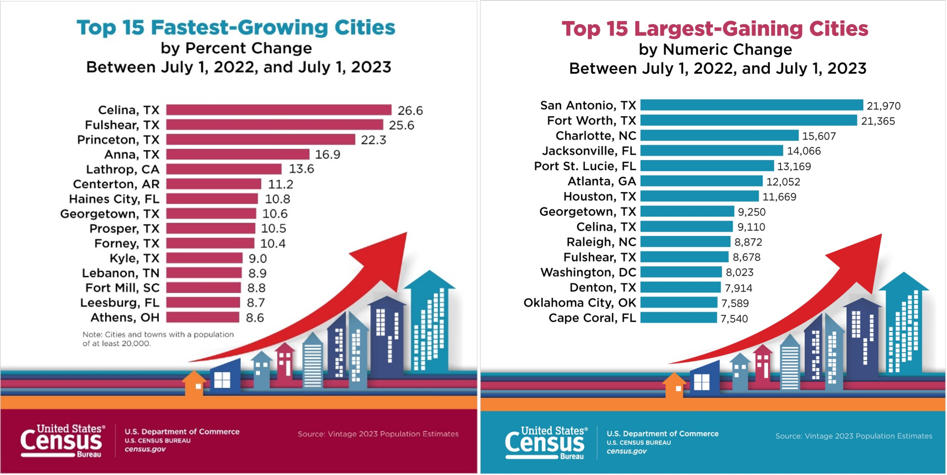
The upward trend in the South’s population growth has been further accelerated by post-COVID-19 migration. According to the U.S. Census, southern cities dominated both the 15 fastest-growing cities and the 15 largest-gaining cities between July 1, 2022, and July 1, 2023 (Figure 1). The distinction between these two groups lies in their composition: the top 15 largest cities on this list are predominantly major urban cities, whereas the fastest-growing cities are mostly small towns that have benefited from larger cities’ migration outflow. Accordingly, this new list of the fastest-growing cities in the U.S. raises an important question: How has the housing price landscape changed in the South since the pandemic?
Figure 1. Top 15 Fastest-Growing Cities and Largest-Gaining Cities between July 1, 2022 and July 1, 2023
Source: U.S. Census Bureau. (2024, May 16).
To answer this question, the Zillow Home Value Index (ZHVI), a smoothed and seasonally adjusted measure of typical home values in the 35th to 65th percentile range, was used to observe the percentage changes in house prices from March 31, 2020, to March 31, 2024, following the World Health Organization’s declaration of COVID-19 on March 11, 2020.
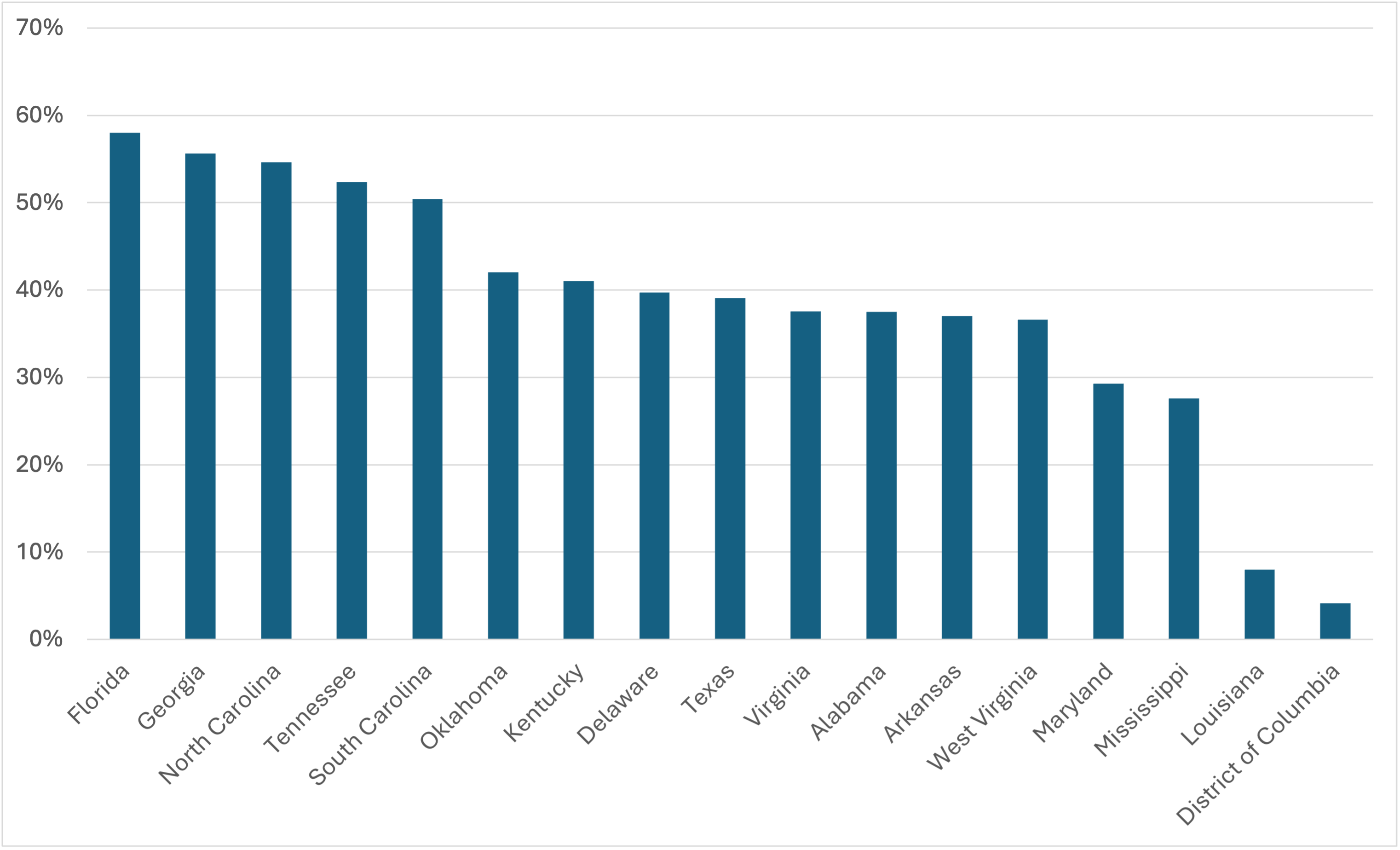
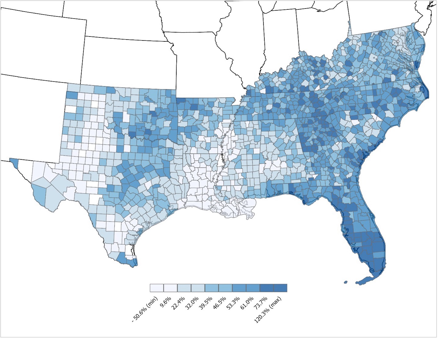
Figure 2 illustrates the percentage changes in house prices across southern states from March 31, 2020, to May 31, 2024. Overall, significant increases were observed in most states, with notable rises exceeding 50% in five states: Florida (58%), Georgia (56%), North Carolina (55%), Tennessee (52%), and South Carolina (50%) since the onset of the pandemic. Conversely, Louisiana and Washington D.C. saw a modest increase of less than 10% during this period, distinct from the upward trends observed elsewhere. In addition, the county-level map (Figure 3) provides geographical insight into the house price landscape. As we can see, house prices in the counties along the Mississippi Delta and a large portion of western and southern Texas counties increased noticeably less or even decreased compared to other regions. These clustered patterns resemble the recent net domestic migration map (2021-2022) from the U.S. Census (U.S. Census Bureau, 2023, March 30). One notable difference is that negative net domestic migration in big cities has rebounded, whereas the net domestic migration around the Mississippi Delta area continues to face challenges, resulting in decreased house prices.
Figure 2.House Price Percentage Changes by State from March 31, 2020, to May 31, 2024, in the Southern Region
Source: Zillow Home Value Index (ZHVI) from March 31, 2020, to March 31, 2024.
Figure 3.House Price Percentage Changes by County from March 31, 2020, to May 31, 2024, in the Southern Region
Source: Zillow Home Value Index (ZHVI) from March 31, 2020, to March 31, 2024 (For some counties (about 30 counties, mostly in TX), data from Feb 28th, 2022, is used due to the absence of past data). Note1: There is a less than 1% likelihood that this clustered pattern could be the result of random chance (Moran’s I: 0.5895, z-score: 90.5022, p-value: 0.0000) Note2: No data is available for the empty counties
So, what exactly does the house price landscape tell us? The sharp increase in house prices across the southern region of the U.S. since the pandemic underscores the immediate need for supportive measures. As housing costs escalate, there is a critical need to prioritize actions that enhance affordability and ensure equitable access to housing. Considering the rising population trend in the South, it is likely that home prices there will keep climbing, exacerbating the issue of housing affordability. In contrast, underserved regions, such as the Mississippi Delta, which are experiencing negative domestic migration trends worsened by the pandemic, may see community development challenges intensify in the future. Therefore, by addressing these dual issues with strategic and supportive approaches, policymakers can promote a more inclusive and sustainable recovery across the diverse landscapes of the South.
References
U.S. Census Bureau. (2024, May 16). Population rebounds for many cities in Northeast and
Recent years have seen several high-profile outbreaks of transboundary animal disease. On average, approximately 0.01% of the world’s cattle population, 0.05% of the world’s swine population, and 0.03% of the world’s poultry population die each year due to global animal disease outbreaks.
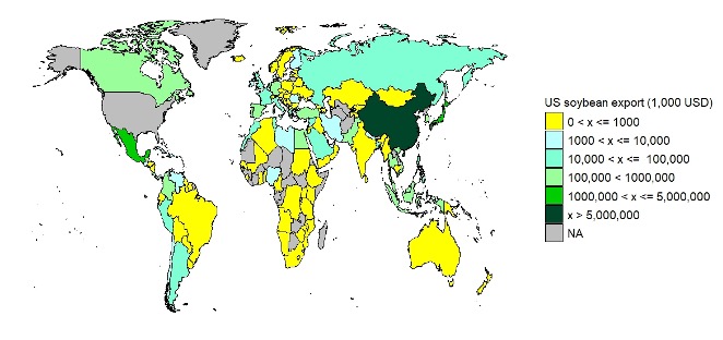
These disruptions cause losses not only in the animal production industry but also in other related industries, such as the feed grain markets. One such upstream industry which is important for Southern U.S. agriculture is the international soybean market. Soybeans are the predominant source of protein in animal feed, and over 95% of global soybean meal production is destined for animal feeding (about 76% of total crush by weight) (Economic Research Service, 2024). Between 2005 to 2020, the U.S. was the second largest exporter of soybeans in the world behind Brazil. U.S. exports account for more than 30% of global soybean trade. The top five destination markets for U.S. soybeans have historically been China, Mexico, Japan, Indonesia, and Germany (Figure 1).
Figure 1: U.S. Soybean Exports, by Destination Market
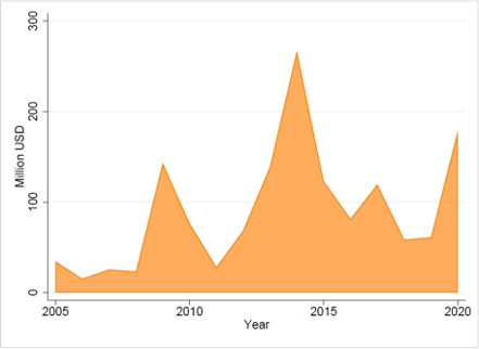
In a recent study, we use a statistical model to examine the losses to global soybean trade due to animal disease (Lwin, Schaefer and Hagerman, 2024). A significant amount of animal deaths within a short period represents a demand-side shock in the feed market, where soymeal is a primary protein source. Our analysis suggests that—on average—more than $96 million in export potential is lost annually due to animal disease outbreaks (Figure 2).
Figure 2: Annual losses in U.S. soybean export potential due to animal diseases
Source: Lwin, Schaefer and Hagerman, 2024
These results should be of interest to policymakers. Historically, animal health policies have focused primarily on compensation to producers of affected livestock, which may include indemnity for animals that die or are depopulated for disease control. Few policies address the risk animal diseases pose to upstream suppliers. Crop insurance programs, if available, may protect grain producers against price declines. However, crop insurance is unlikely to address additional costs of storage or quality loss for grain that must be stored for longer periods of time. Policy efforts to enhance supply chain resilience should consider the ripple effects of animal disease-related disruptions on related industries.
References
Economic Research Service, USDA. 2024. “International Baseline Projections.” Accessed: 2024-02-02.
Lwin, Wuit Yi, K. Aleks Schaefer, and Amy D. Hagerman. 2024. “Animal Disease Outbreaks and Upstream Soybean Trade.” Food Policy, 127: 102685.