Blog

  • The Disparity Between Crop Prices Received and Input Prices Paid

    The Disparity Between Crop Prices Received and Input Prices Paid

    The United States Department of Agriculture National Agricultural Statistics Service (USDA-NASS) releases monthly indexes for input prices paid and output prices received. These indexes include collecting survey responses for output and input prices for agricultural production, crops, livestock, and food commodities. The spread between these two indices often helps understand where farmers are getting price squeezed and how their profit margins are impacted. Current farm income instability from inflationary pressures, high interest rates, and several supply chain disruptions (e.g., the Russian-Ukraine war and Panama/Suez Canal) are forcing farmers to pay higher input costs while receiving lower commodity prices, emphasizing the need to consider these indexes into the future. 

    These price indices measure the change in prices paid (and received) relative to a point in time—2011 in this case (Figure 1). The base year is often chosen during a time without prevailing inflation or major supply chain disruptions (Schulz, 2022). 2011 was a good year for agricultural production and profitability. As such, using 2011 as a base year is a way to highlight how better or worse-off agricultural producers are compared to a good year. 

    Figure 1. Crop Output Prices Received vs. Input Prices Paid
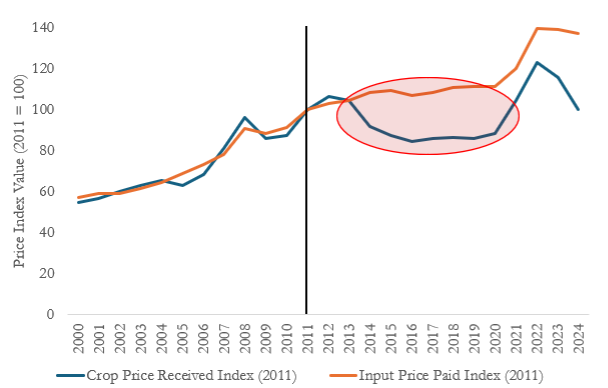
    Figure 1 compares the annual index value from 2000-2024 for the two indices with 2011 as the base year. The price received index in 2012 was 102.8%, meaning that the crop price received, on average, in 2012 was 2.8% higher than in 2011 (base year = 100%). The red circle in Figure 1 shows the beginning of a divergence between input and output prices. In 2013, when writing the 2014 farm bill, the index for input prices paid was almost exactly the index for output prices received. This is where most of our current farmer safety net support stems from, and since then, we’ve seen a major divergence in the two indices, with the widest gaps between 2014 – 2020 (USDA-NASS). From 2021 – 2022, we saw both indices increase, but the gap remained, and the divergence has grown wider in 2023 and 2024 due to declining commodity prices. 

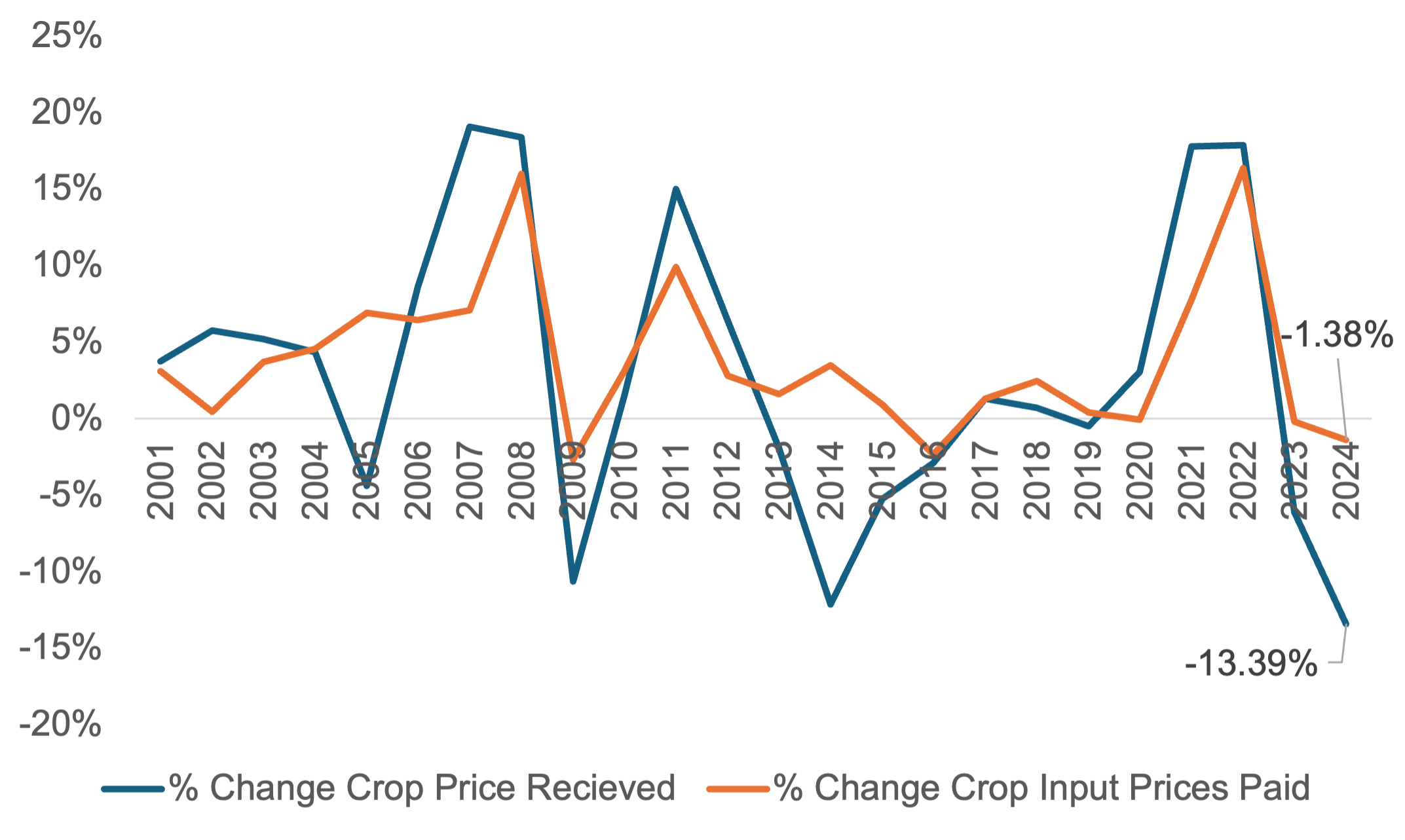
    Another way to view the indices is to calculate how they change year to year. Figure 2 plots the same indices as Figure 1 but shows the yearly change between the index values. Using this percentage change helps producers understand 1) the volatility of crop output prices and 2) the magnitude of change as compared to the previous year. A key takeaway is that input prices are less volatile (in terms of yearly % change) than output prices. Secondly, the percentage change in crop output prices between 2023 and 2024 (-13.8%) is much larger than the percentage decrease in input prices (-1.38%) during that period.

    Without any relief in the form of improved crop prices received, figure 1 suggests farmers will continue to suffer from cost/price squeezes and eroding profit margins. Further, figure 2 shows the magnitude of that spread between the indices in Figure 1; if input and output prices continue this trajectory, an improved farm safety net will be warranted. This will be at the forefront of every producer’s mind, with ongoing Farm Bill debates in 2024.  

    Figure 2. Year-over-Year % Change in Input and Output Crop Prices

    References

    Schulz, L. (2022). Disentangling Input and Output Price Relationships. Retrieved from: https://www.extension.iastate.edu/agdm/articles/schulz/SchSep22b.html

    The Observatory of Economic Complexity (OEC). (2024). Fertilizers in Russia. Retrieved from: https://oec.world/en/profile/bilateral-product/fertilizers/reporter/rus

    USDA-Economic Research Service (2024). Farm Sector Income & Finances: Highlights from the Farm Income Forecast. Retrieved from: https://www.ers.usda.gov/topics/farm-economy/farm-sector-income-finances/highlights-from-the-farm-income-forecast/

    USDA- Economic, Statistics, and Market Information System. (2024). Agricultural Prices. Retrieved from: https://usda.library.cornell.edu/concern/publications/c821gj76b?locale=en


    Loy, Ryan, and Hunter Biram. “The Disparity Between Crop Prices Received and Input Prices Paid.Southern Ag Today 4(28.3). July 10, 2024. Permalink

  • Falling Corn Prices, Higher Calf Prices

    Falling Corn Prices, Higher Calf Prices

    Two big USDA reports in the last week have boosted livestock prospects at the expense of corn prices.  The annual Acreage report included larger-than-expected corn acres which put downward pressure on corn prices. The report listed corn acres at 91.5 million acres which was 1.4 million acres higher than the March Prospective Plantings report projected. After corn prices surpassed $6 for the 2022/23 marketing year, prices fell below $5 for the current marketing year, and are projected to be closer to $4 for the 2024/2025 marketing year. 
     
    While higher than previously projected, corn acres will be slightly lower than 2023 totals. However, good growing conditions are supporting higher yield expectations when compared to 2023. The latest WASDE report included a yield estimate of 181 bushels per acre which would be higher than the 177.3 from a year ago. Stronger yields could lead to corn production for 2024 not being far off from the 2023 total. 
     
    Also released last week was USDA’s Quarterly Grain Stocks Report which includes estimates of corn stocks held on farms and in elevators. Total corn stocks on June 1st were estimated to be 5 billion bushels, up 22 percent from 2023 and the highest June 1 total since 2020. Most of these stocks are still being held on farms as farmers await better pricing opportunities. But, the old common problem arises of holding stocks while supplies grow and prices continue to fall.  On farm corn stocks were just over 3 billion bushels, which is roughly 800 million more than last year and is the largest June 1 total since 1988. 
     
    Overall, the news is positive for livestock producers. The simple takeaway is that corn production and stocks are expected to be plentiful, and corn prices are back to lower levels after surging a few years ago. This should continue to bring relief to livestock feed costs and reduce the cost of gain for cattle.  This year’s corn crop is not in the bin yet, so production risks remain that could influence price. Falling corn prices should continue to push calf prices further into record territory.  Returns to hog and poultry production will get a much needed boost from lower feed costs.

    Maples, Josh, and David Anderson. “Falling Corn Prices, Higher Calf Prices.” Southern Ag Today 4(28.2). July 9, 2024. Permalink

  • Revenue Protection Weighted Average Coverage Levels by County and Crop

    Revenue Protection Weighted Average Coverage Levels by County and Crop

    Producers make several important marketing and risk management decisions throughout the year. One of the most important decisions is the choice of coverage levels when purchasing crop insurance. Revenue Protection (RP) – by far the most popular plan of insurance – provides an indemnity if realized revenue (combination of yield and price) drops below the guarantee (or a percent of expected revenue) for the insured unit. RP coverage levels range from 50% to 85% of expected revenue, increasing in 5% increments. Producers must weigh the choice of varying RP coverage levels against the changes in premium costs. Premium costs vary and consider factors such as the risk of loss for the insured crop in the specific county, coverage level, insurance product purchased, and production practices. This article examines the weighted average coverage level (WACL) by county and crop from 2011-2022 for corn, cotton, soybean, wheat, and peanut RP insurance plans. RP insurance plans from 2011 to 2022 covered 88% of all insured acres for corn, cotton, peanuts, soybeans, and wheat (USDA Summary of Business). The WACL is calculated as RP coverage level multiplied by acres insured for the coverage level divided by total RP acres insured for each county crop and year.

    Corn

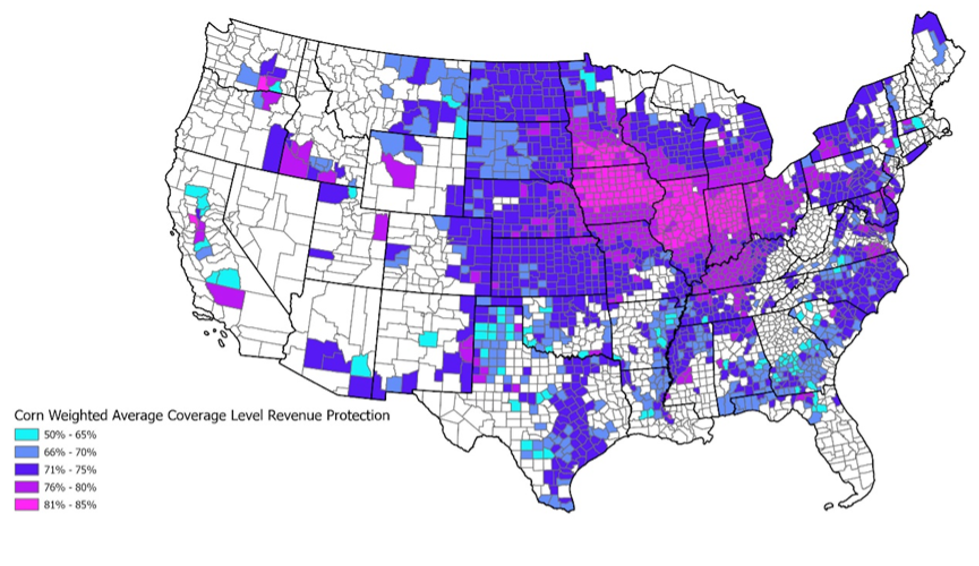
    The Corn Belt states of Indiana, Illinois, and Iowa show most counties have a WACL of 81% to 85%, indicating higher insurance coverage purchases. Most counties in North Dakota, South Dakota, Nebraska, and Kansas exhibit a WACL of 71% or greater. However, there is more variability in the southern and eastern states, with coverage levels generally lower than in the Midwest.

    Figure 1. Corn Acre-Weighted Average Coverage Level Revenue Protection 2011-2022

    Data Source: USDA RMA Summary of Business

    Cotton

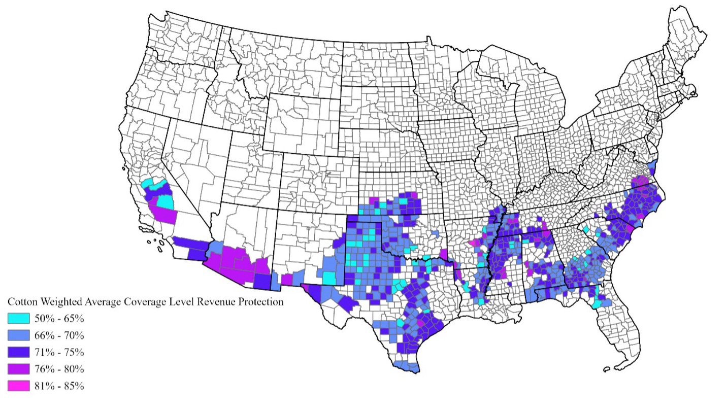
    Southern Arizona has a concentration of 76% to 80% WACLs for cotton, while the majority of Western Oklahoma and Texas counties have a WACL for cotton of 66%-70%. The rest of the south’s cotton production is concentrated along the Mississippi River, the east coast, South Georgia, and South Alabama with a 71-75% WACL being the most prominent coverage level. Nationally, there are very few counties with a WACL above 80% for cotton.

    Figure 2. Upland Cotton Acre-Weighted Average Coverage Level Revenue Protection 2011-2022

    Data Source: USDA RMA Summary of Business

    Peanuts

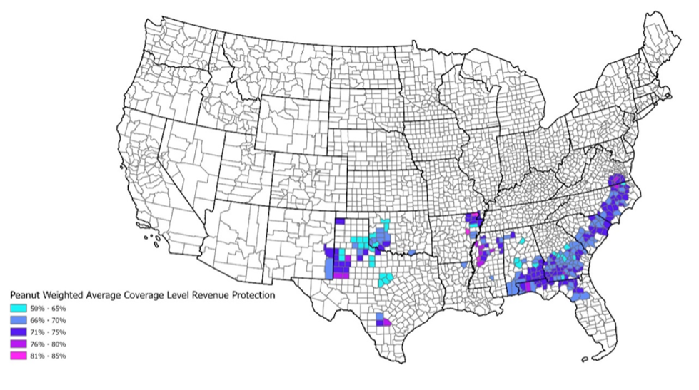
    The southern regions of Alabama, Georgia, and the eastern Carolinas show a WACL between 66% and 75%. About half of the counties in Northeast Arkansas and Northwest Mississippi have a WACL of 76% or higher. The counties along the border of Western Oklahoma and Texas have lower WACLs, while those along the border of West Texas and Eastern New Mexico mainly have WACLs of 71% or higher. Like cotton, peanuts have few counties with WACLs that exceed 80% – fewer than twenty counties have WACLs greater than 76%. 

    Figure 3. Peanuts Acre-Weighted Average Coverage Level Revenue Protection 2011-2022

    Data Source: USDA RMA Summary of Business

    Soybeans

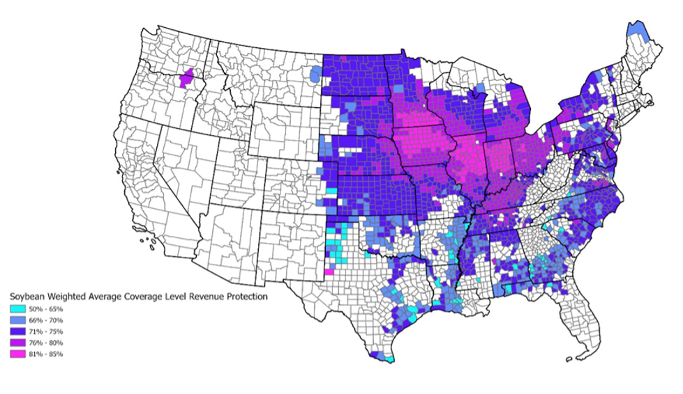
    Trends for soybeans mirror those for corn, with counties in Ohio, Indiana, Illinois, Iowa, and Kentucky showing WACLs of 76% or higher, with many reaching 81% or higher. From North Dakota to Kansas, counties have WACLs of 71% or better. In the southern states, the WACL varies significantly.

    Figure 4. Soybeans Acre-Weighted Average Coverage Level Revenue Protection 2011-2022

    Data Source: USDA RMA Summary of Business

    Wheat

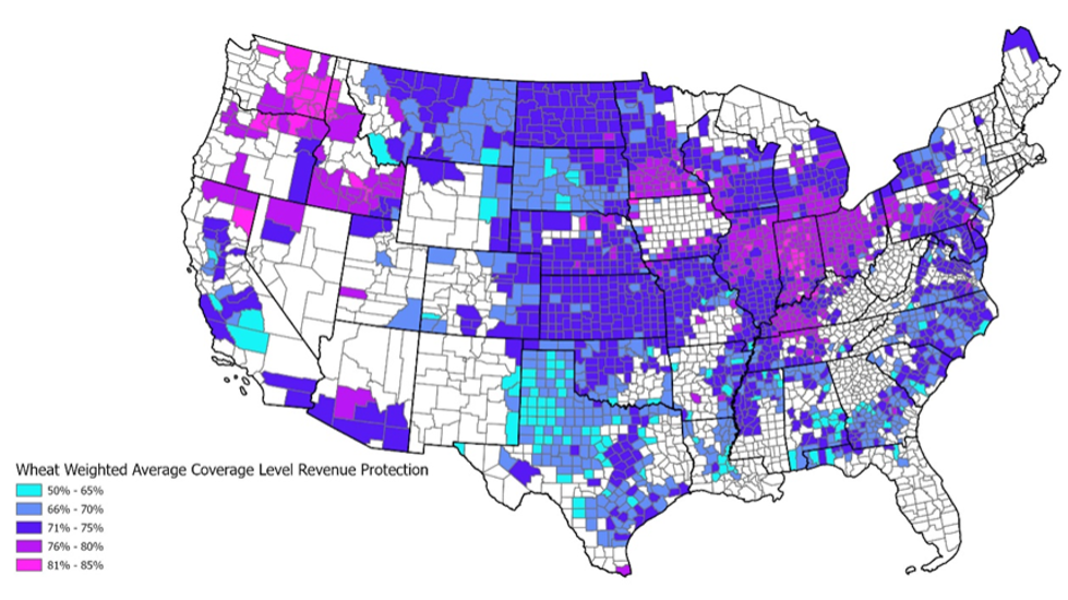
    Northwestern states and parts of the Midwest exhibit WACLs of 76% or greater. In Texas, many counties show lower WACLs, ranging from 50% to 70%. Wheat production varies by season (spring or winter) and type (hard, soft, and durum). Wheat production in the northwestern states is typically soft spring wheat, whereas Texas wheat is mostly hard red winter wheat that produces lower yields than soft wheat. 

    Figure 5. Wheat Acre-Weighted Average Coverage Level Revenue Protection 2011-2022

    Data Source: USDA RMA Summary of Business

    Since the early 1990s, buyup coverage levels for crop insurance have trended higher (Smith, 2015). From 2011 to 2022, across commodities there is greater variability in WACLs in the South than the Midwest and Northern Plains. Variability in WACLs by crop and region highlights differences in risk levels, risk preferences, insurance premiums, and production costs. Regions with higher WACLs often have more consistent yields; regions with lower WACLs typically face higher premium costs due to greater production variability. Understanding trade-offs in risk and premium cost can help producers determine the correct RP insurance coverage level to meet their specific risk management needs.

    References and Resources:

    Biram, H.D. 2024. The Fundamentals of Federal Crop Insurance, University of Arkansas. Link

    Smith, S.A., J. Outlaw, and R. Tufts. 2015. Surviving the Farm Economy Downturn. Chapter 10. Crop Insurance: Basic Producer Considerations. https://afpc.tamu.edu/extension/resources/downturn-book/.

    USDA Risk Management Agency. Summary of Business. https://www.rma.usda.gov/SummaryOfBusiness


    Duncan, Hence, and Aaron Smith. “Revenue Protection Weighted Average Coverage Levels by County and Crop.Southern Ag Today 4(28.1). July 8, 2024. Permalink

  • Is the Current CSA Model Sustainable? A Lesson from Korea

    Is the Current CSA Model Sustainable? A Lesson from Korea

    The popularity of Community-Supported Agriculture (CSA) has been on a downward trend for over 20 years. As such, the continuous decline of CSAs raises the question of whether their traditional business model can compete with other local food sources. Since the first CSA program was introduced in 1986, CSAs have not changed their core model; farmers and consumers maintain a direct relationship, ensuring financial support for the farmers while providing members with locally grown food. Typically, CSA members pay a seasonal up-front fee ranging from $400 to $800 in exchange for predesignated boxes of raw ingredients, which can be picked up or delivered. Though many CSAs have partially modified their model with up-front pricing policies and CSA box options, their core model has yet to change since its inception. Meanwhile, CSAs became the least favorable option for local food customers (Seo & Hudson, 2023). Many larger retailers provide local food with greater accessibility, diverse selections, and entertainment options like live music. Similarly, farmers’ markets offer fresh local food with a strong emphasis on community engagement & support, and various entertainment, which CSAs typically lack. Thus, the continuous diminishing of CSAs suggests that they need to reconsider their outdated business model to remain competitive and sustainable among other local food sources.

    However, the local food model in South Korea sheds some light on how CSA farmers could better position themselves among local food sources. In Korea, numerous small local food shops run by small cooperatives effectively bridge the gap between micro farmers and customers in rural communities. The common thread among these local food shops is their utilization of the Wanju Local Food Cooperative‘s local food model. This model won awards at the Milan Urban Food Policy Pact (MUFP) in Governance for “Local Food No. 1 Project” in 2018 and in Social and Economic Equity for “Equal Healthy Food for All: Wanju Type Food Plan” in 2022. It was also praised by the Food and Agriculture Organization (FAO) as a successful regional food localization strategy (FAO, 2017). As such, the Wanju Local Food Cooperative is an excellent example of how CSAs can revive themselves and become popular once again.

    When the Wanju Local Food Cooperative initially started, they used the traditional American CSA box delivery model. Though they still offer CSA boxes to customers, their success began with their first offline local food shop in 2012, right around the same time that the number of CSAs in the United States started to decrease. To launch their first offline shop, the cooperative created contracts with 1,011 local farmers and developed detailed crop production plans to offer customers a small but diverse selection of produce. Since then, the shop has functioned as an open market for micro farmers who have completed training courses and submitted production plans to sell their produce freely. To ensure the highest quality products, the Wanju Local Food Cooperative maintains a strict list of policies, including: 

    • Fresh produce must have been harvested the same morning that it is brought to the market for sale

    • Farmers independently pack, display, and price their own produce

    • Unsold produce is either discarded or returned to the original farmer

    • Farmers pay a 10% commission fee to the cooperative 

    Furthermore, the cooperative managing the local food shop extends its services to restaurants within the shop, provides online shopping options, offers food processing facilities to farmers, and even enhances community engagement through agrotourism initiatives such as farm tours and cultural events. As a result, it is common to see residents and tourists flock to the shop early in the morning to buy the freshest locally grown produce and enjoy the restaurants serving local food. This successful local food model spread nationally and became a popular community support model throughout Korea. Because the local food shops offer a variety of the freshest produce, good accessibility in residential areas, competitive prices from competition between farmers, entertainment events, and no exclusive membership or up-front fee policy, these local food shops have established their unique place among local supermarkets and farmers’ markets.

    The success of the Wanju Local Food Cooperative underscores two pivotal elements for an effective local food model: minimizing market entry barriers for small farmers and offering a diverse range of produce to customers under one roof. Many small farmers struggle to access markets due to quantity constraints, which deter both existing farmers and potential newcomers. The Wanju Local Food Cooperative has overcome this challenge through its open-market approach.Additionally, while local food consumers do seek shopping experiences that support local farmers and foster community engagement, their primary desire is a convenient location to purchase their weekly groceries. In contrast, the traditional CSA model often receives criticism for its limited selection. However, the Wanju Local Food Cooperative addressed this by coordinating farmers’ production plans to offer a broader array of produce, prioritizing variety over quantity to fulfill the objective of convenient grocery shopping. Therefore, if CSAs in the United States seek to remain competitive with other local food sources and genuinely support community farmers to be more than just a produce box delivery service, they should reconsider their traditional approach to running their organizations. 

    References

    Food and Agriculture Organization of the United Nations. (2017). Wanju: Supporting Local Agriculture 

    through Direct Food Marketing, Milan Urban Food Policy Pact Category: GovernanceFood and Agriculture Organization of the United Nations (FAO). https://openknowledge.fao.org/handle/20.500.14283/ca0491en

    Seo, F., & Hudson, D. (2023). Attributes that Influence Consumers’ Preferences for 

    Choosing Locally Grown Food Sources During and After the COVID-19 Pandemic. Journal of Agricultural and Applied Economics. 2023;55(4):626-650. doi:10.1017/aae.2023.27


    Seo, Frank. “Is the Current CSA Model Sustainable? A Lesson from Korea.Southern Ag Today 4(27.5). July 5, 2024. Permalink

  • Estate Transition Planning

    Estate Transition Planning

    The University of Tennessee Institute of Agriculture hosted the 2024 Beef Improvement Federation Conference two weeks ago. One session that spurred on great conversations was estate transition planning and what that entails. Table 1 displays the Southern Ag Today states and the age break downs of total producers. Kentucky has the highest percentage of producers that are under the age of 35 (10%). For the age range of 35 years to 64 years, all states have over 50% of their producers in this category. But, six states (TX, VA, MS, GA, SC, and FL) have 40% of their producers in the 65 years of age and older category, with Mississippi having the highest percentage at 42%. Farm management is often thought about only from a financial performance (income statement, balance sheet, cash flow statement) standpoint, but sound farm management also includes planning for the future, including estate and management transitions. 

    A large number of producers in the Southern region are potentially nearing retirement or are over the age of 65 years. This would suggest that estate transition planning should start becoming a priority. If the goal of the farm is to stay a farm, then at some point in the future, the farm will change hands. Transition planning can become a huge task if no plan has ever been thought about or developed. Often, producers indicate that they don’t know where to start. That is understandable. Thus, a good starting point could be, “What is adequate retirement income?” Building upon this question could solve questions like: “What are my lifestyle costs? Will costs change in retirement (life care)? How much income will come from social security, pensions, savings, investments, and the farm?” Each farm is different and has diverse challenges like trusts, multiple families/individuals in the operation, debt amounts, urban encroachment, and many more. 

    However, starting the conversation is the most important step for everyone involved in the process. The key to this falls on the shoulders of the parent(s). Not only is it awkward for the child, or children, to start this conversation, but if there are multiple children and one takes the lead, it can have unintended consequences. But just initiating the conversation is the start. Throughout the process, there are many tools that can be utilized: a will, power of attorney, advanced healthcare plan, healthcare agent, trusts, insurance, letter of last instruction, and easements. While the previous sentence has a lot of moving parts, having a team of professionals could aid in the process and make it easier. The team could include an attorney, accountant, financial planner, lender, extension educator, business consultant, and communication specialist.

    The topic of estate transition is diverse, and it looks different for every operation, but starting the process is never the wrong step. This article only scratches the surface, but below are resources available to you to start. 

    University of Tennessee: Farmland Legacy- https://farmlandlegacy.tennessee.edu

    University of Minnesota- https://agtransitions.umn.edu

    Iowa State University- https://www.extension.iastate.edu/bfc

    Table 1. Age Group Break Down of Total Producers for Southern Ag Today States

    Percent of Producers in Age Group
    StateTotal Producers<3535-6465 and Older
    TX402,8766%52%41%
    OK124,7439%53%37%
    AR67,4259%54%36%
    LA42,5518%54%38%
    KY119,13210%55%35%
    VA67,7988%52%41%
    TN107,8177%53%39%
    NC72,4799%54%38%
    MS52,0257%51%42%
    AL62,7778%53%39%
    GA67,0827%53%40%
    SC38,0978%51%41%
    FL79,2537%53%40%
    (Source: 2022 Ag Census)

    Martinez, Charley, and Kevin Ferguson. “Estate Transition Planning.Southern Ag Today 4(27.3). July 3, 2024. Permalink