Blog

  • Using Risk Preference to Inform Crop Insurance Decision-Making

    Using Risk Preference to Inform Crop Insurance Decision-Making

    Crop Insurance decisions are closely tied to farmer’s risk preferences. Each producer faces different circumstances and has a different risk tolerance. Some producers prioritize revenue stability and opt for higher coverage levels and choose optional units for more targeted coverage. Conversely, others may be able to tolerate more risk and choose lower coverage levels or utilize basic or enterprise units in exchange for lower premiums. Crop insurance decisions can be overwhelming as the full suite of protection also involves choices on the FSA programs (ARC or PLC), crop insurance product, unit structure, and coverage level. Each of these choices need to made taking into account producer risk preference. 

    In discussing the effects of risk on crop insurance decisions, we use an online application, “Crop Insurance Decision Maker, ” which can be found here. A set of example results for Christian County, Kentucky, can be seen in Figure 1. In our case example, we look at insurance on non-irrigated corn acreage using enterprise units. The case example illustrates that as the coverage level increases, average net revenues increase. Among the three main crop insurance products (YP, RP, RP-HPE), Revenue Protection (RP) consistently yields the highest net revenues, followed by Yield Protection (YP) and then Revenue Protection with a Harvest Price Exclusion (RP-HPE). This suggests that on the example farm, higher levels of coverage generally lead to better average net revenues ($/acre), with RP providing the most significant benefit. 

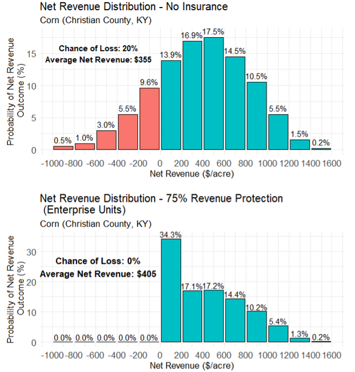
    The fact that average net revenue increases with coverage level may seem counterintuitive but is evidence of the effect of a reduction in the actuarially fair insurance premium. To discuss this point, we use Figure 2, which compares the net revenue distributions for Christian County, Kentucky, utilizing no crop insurance and a 75% RP plan utilizing Enterprise Units. Figure 2 indicates that with no crop insurance, a producer faces a 20% chance of net revenues less than zero which is the downside risk a producer wants to minimize or eliminate. Conversely, the 75% coverage level in this example eliminates the downside risk of negative net revenues while slightly reducing the likelihood of larger returns. Due to the protection offered, net income increases on average. That is, the downside risk reduction outweighs the reduction in the upside potential driven by the producer paid premium.

    Our comparisons in Figure 1 and Figure 2 should be considered for each insurance decision. Net revenue probabilities change each time a crop insurance product, unit structure, or FSA program is changed. Each producer needs to determine their risk preference as under-insuring could leave the producer vulnerable to losses. Still, over-insuring could limit net income in years when indemnities are not triggered. The “Crop Insurance Decision Maker” aims to make these choices easier. It is important to note that the effects of each crop insurance decision change by county depending upon premiums, and the results for Christian County, Kentucky, may not hold for your operation.

    Figure 1: Crop Insurance Decision Maker Web Application Output
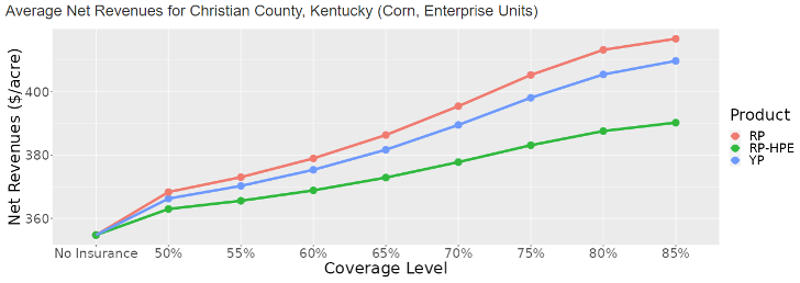
    Figure 2: Net Revenue Distribution for No Insurance VS a 75% Revenue Protection Plan using Enterprise Units
    References

    Biram, Hunter D., et al. “Mitigating price and yield risk using revenue protection and agriculture risk coverage.” Journal of Agricultural and Applied Economics 54.2 (2022): 319-333.

    Maples, William E., et al. “Impact of government programs on producer demand for hedging.” Applied Economic Perspectives and Policy 44.3 (2022): 1126-1138.


    Serrano, Enil, Grant Gardner, and Hunter Biram. “Using Risk Preference to Inform Crop Insurance Decision-Making.Southern Ag Today 4(29.3). July 17, 2024. Permalink
  • Retail Meat Prices Ease a Little

    Retail Meat Prices Ease a Little

    Nestled down in the bowels of the Consumer Price Index (CPI) data that is released each month is the retail price of beef, pork, and chicken.  Each have reached record highs at some point in the last couple of years adding to overall food price inflation.  The latest CPI data for meats indicated some stabilization or decline in meat prices.  

    First off, it’s worth remembering what this data represents.  It is the price of various cuts of beef, pork, and chicken reported from grocery stores during the second week of the month.  The data does not include special features, sales, in store coupons, or customer loyalty card discounts.  As a grocery store price, it does not include meat prices at restaurants. 

    Meat prices (and production for that matter) exhibit a considerable amount of seasonality.  Both supply and demand factors contribute to price seasonality.  For example, on the supply side, pork production tends to peak in the Fall after hitting its seasonal lows in Summer.  Tighter supplies in the Summer would suggest that prices should peak in Summer.  But, on the demand side, individual cuts may peak at different times of the year, for example, hams at the holidays or grilling season favorites.  Economists often compare the most current price to those of last year at the same time, simply to account for normal seasonality of prices.  But, for many consumers thinking about inflation a more useful comparison might be to last month or the last couple of months to account for the trend in prices.

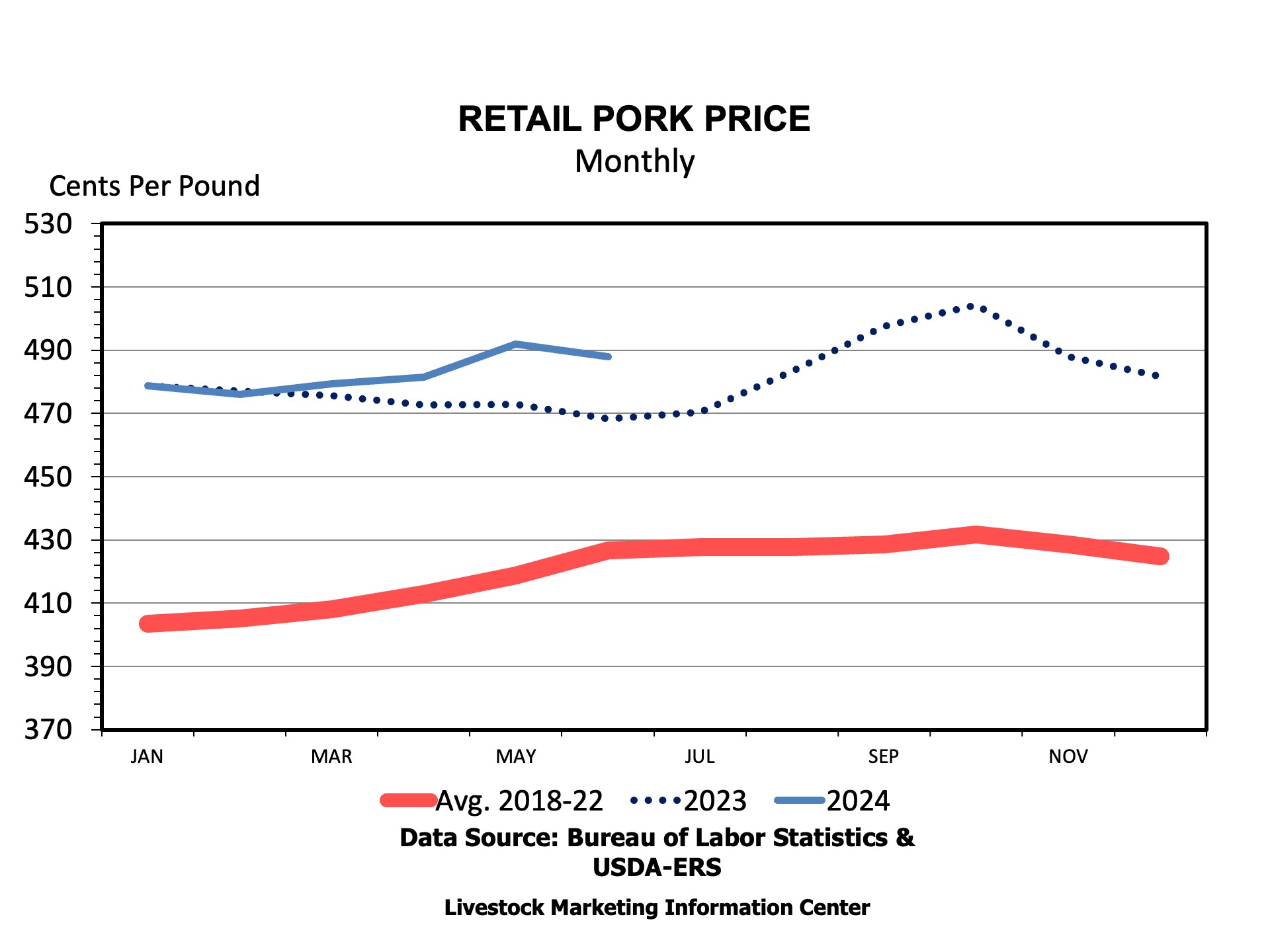
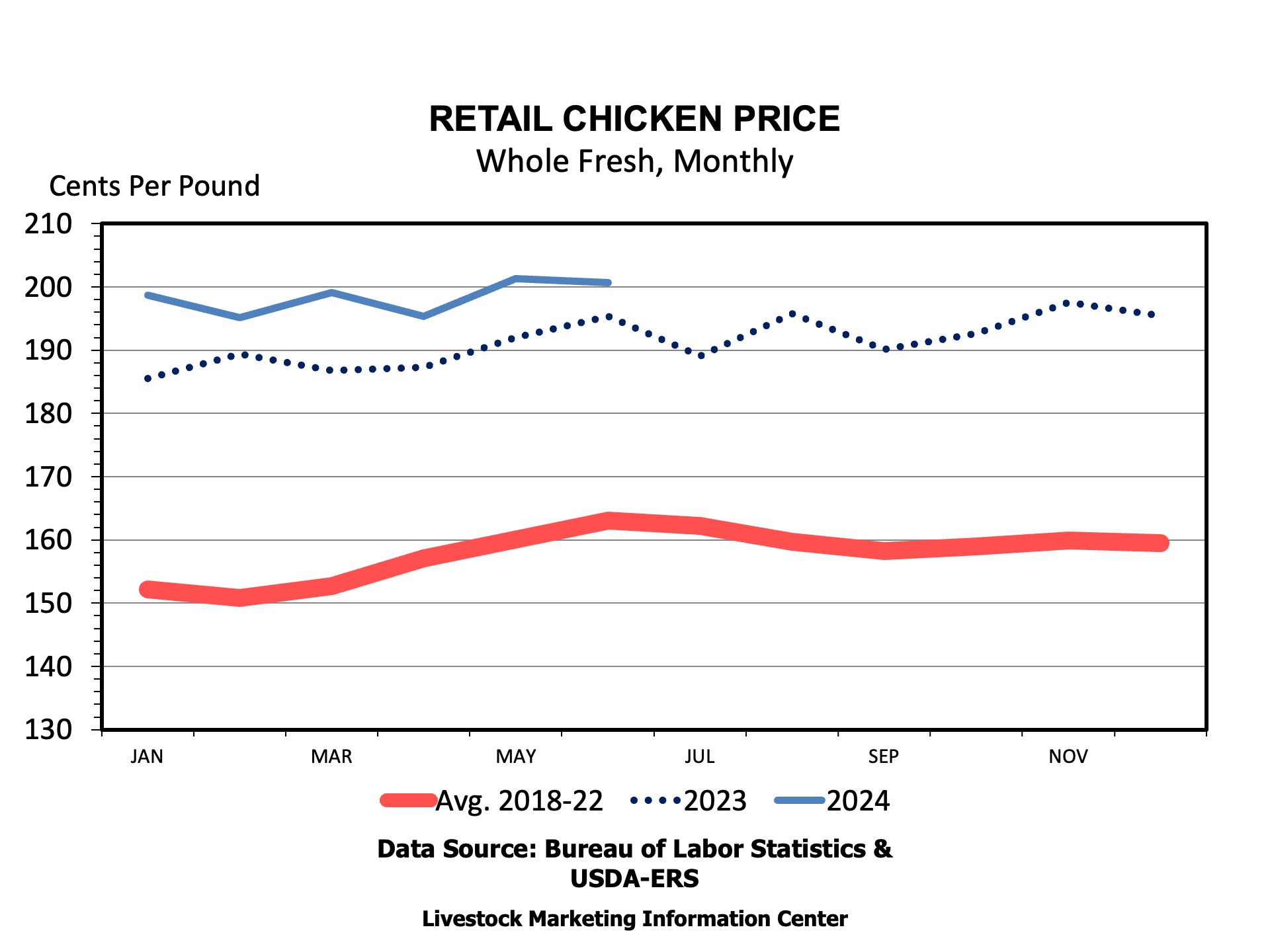
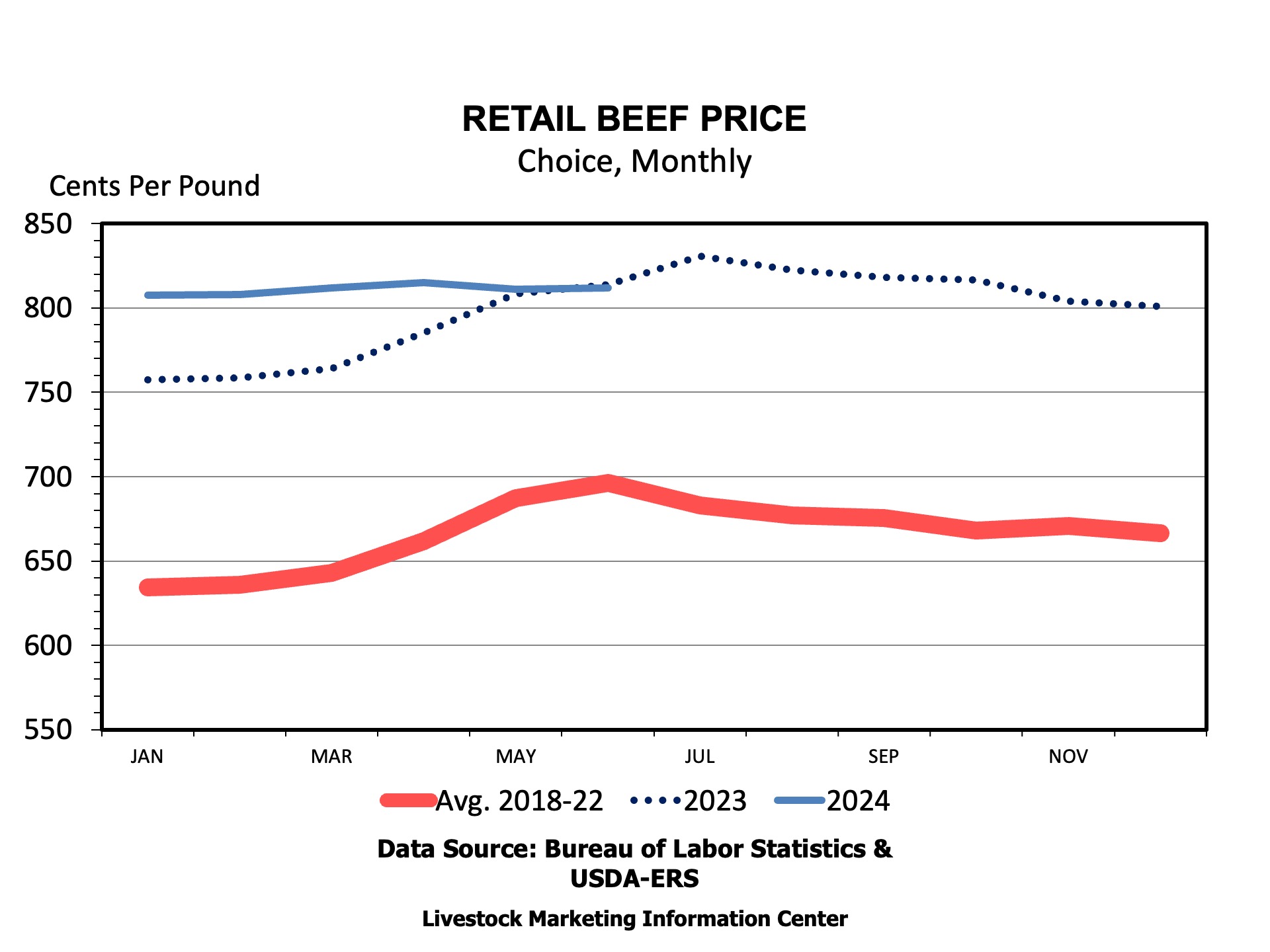
    The latest data represents June prices across the U.S.  The Choice beef price in June was $8.119 per pound, less than 1 cent per pound higher than May.  So far this year, Choice beef prices peaked in April at $8.151 per pound.  Compared to a year ago, beef prices were about 2 cents lower per pound.  Pork prices totaled $4.88 per pound in June compared to $4.919 per pound in May and $4.684 per pound in June of last year.  Chicken prices are reported in two ways: as a whole, fresh bird retail price or as a composite price made up of various cuts.  The composite retail price was $2.403 per pound in June compared to $2.44 in May and $2.504 in June 2023.  

    On the whole, the latest retail meat price data indicates some easing of meat price inflation in June.  Some recent falling cutout values for beef and pork related to more production of both relative to last year could be part of the reason for lower prices.  Some consumer push back against high prices could have pressured prices lower as well.  Retail prices the rest of the year will be affected by reduced beef supplies and more pork and poultry.


    Anderson, David. “Retail Meat Prices Ease a Little.Southern Ag Today 4(29.2). July 16, 2024. Permalink

  • The Net Short Hedge Fund Position in ICE Cotton Futures

    The Net Short Hedge Fund Position in ICE Cotton Futures

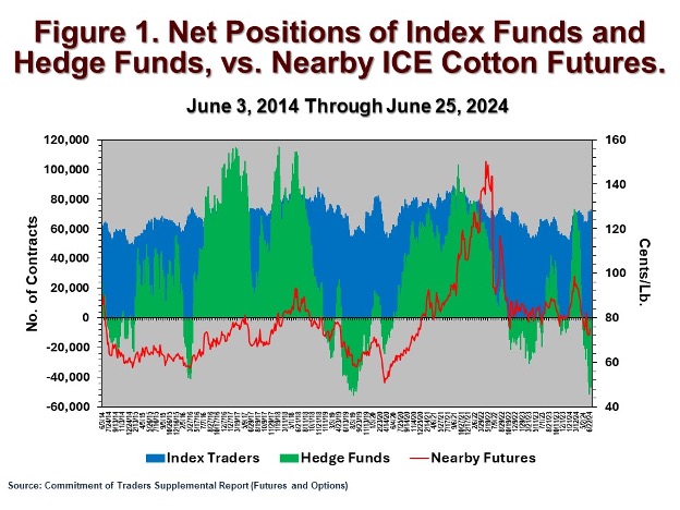
    Hedge funds or “managed money” refers to financial client money that is invested in commodity futures, stocks, bonds, and other investments. Figure 1 shows varying levels of hedge fund investment in ICE cotton futures over the last ten years, either positioned as bullish net longs (i.e., upward pointing green areas) or bearish net shorts (i.e., downward pointing green areas).  In contrast, the blue colored graphed area of Figure 1 reflects the more stable, long-only positioning of index funds. The latter tend to buy and hold nearby futures contracts, and then roll forward as those contracts mature.

    Statistically, net long/short positioning of hedge funds is directly associated with higher/lower ICE cotton futures. Past statistical modeling indicates that a 1.9-cent decline in the most active cotton futures price was expected for every 10,000-contract decrease (or increase) in the hedge fund net long (net short) position (https://www.farmprogress.com/cotton/cotton-spin-hedge-funds-revisited ).  Looking at the most recent price decline, the hedge fund net long position peaked at 73,230 contracts on February 27, 2024, when nearby ICE cotton futures settled at 98.80 cents per pound.  This net long position changed to a 51,442 net short position, a total change of 124,672 contracts and associated with a 72.76-cent settlement on June 18 in nearby ICE cotton futures.  The previous statistical relationship implies that 23.56 cents of the total 26.04 cent decline in nearby ICE cotton futures is associated with bearish hedge fund adjustment, all other things being equal. 

    How long will the current net short position last?  Figure 1 highlights that net short positioning is less frequent than net long positioning.  Over the ten years graphed in Figure 1, only 156 weekly observations involved net short positioning while 370 weekly observations involved net long positioning.  Practically speaking, speculating on the size of an establishing, growing crop during the summer is a bit of a risky gamble.  This dynamic may encourage caution on the part of short speculators during the growing season.  Such behavior could also be the basis of a short covering rally in the event of reduced acreage expectations, bad weather, or negative production scenarios.  Short covering is where hedge fund managers buy back their outright short speculative positions as a result of changing (i.e., more bullish) expectations and/or pre-set buy stop orders.  The liquidation of a large net short position can thus lead to a cascade of buying, referred to as a short covering rally.


    Robinson, John. “The Net Short Hedge Fund Position in ICE Cotton Futures.Southern Ag Today 4(29.1). July 15, 2024. Permalink

  • Natural Disaster Insurance and Markets Under Pressure: New Challenges to Managing Risk in Rural Communities

    Natural Disaster Insurance and Markets Under Pressure: New Challenges to Managing Risk in Rural Communities

    In October of last year, The Progressive Corporation announced that it would not be renewing about half of its homeowner’s insurance policies in the state of Florida. The notice went into effect last month, with letters going out to homeowners stating, 

    Dear Policyholder, your policy will expire at 12:01 on July 1, 2024, for the following reasons. After careful consideration we are unable to offer you a renewal policy due to a reduction in our hurricane exposure. Please contact your agent to find replacement coverage”.

    They were not the first insurer to do so and are not expected to be last. Damage from natural disasters across the Gulf Coast, whether in the form of windstorms, flooding, or hail, has led to a rise in the payouts insurers are making to their policyholders. The Insurance Information Institute’s 2023 annual report wrote of the 28 US weather events exceeding damages of $1 billion, breaking a previous record of 22 in a single year. These disasters led to total insured losses of approximately $60 billion in 2023 (Insurance Information Institute, 2023). To remain solvent these insurers are managing through two courses of action, passing on costs via increased premiums for consumers, and exiting regions where the risk is deemed too high to justify any premium at all. With insurance a requirement for almost all property under lien (commercial, residential, or agricultural), a relatively less stable insurance market threatens a community’s very ability to build capital, by threatening its ability to take advantage of credit. 

    Among the policy proposals intended to shore up these markets are new allowances for premium hikes, adaptation policies such as more stringent building compliance codes, and an increased reliance on reinsurance and “catastrophe bonds” intended to spread out risk among global investors. New research has studied the threat of adverse selection in these markets, particularly as it relates to one’s own perceived vulnerability to a natural disaster (Wagner, 2022). In short, natural disaster insurance markets are adversely selected if homeowners with a higher willingness to pay for insurance are also more costly to insure. Akin to the problem health insurers have with smokers seeking insurance without disclosing their smoking, those homeowners who feel most at risk to natural disasters are the most likely to seek insurance for them. When this is the case, an increase in premiums tends to crowd out those with the lowest willingness to pay, which also tend to be those with the lowest risk among policy buyers. If this occurs, no progress is made toward an insurer’s goal of improving the cost/risk profile of their portfolio, while making insurance more expensive for those who remain insured. The administrators of the National Flood Insurance Program considered this a top concern during their latest meetings on long-term authorization (Wagner, 2022).

    Reinsurance has long been an effective tool for disseminating local risk to a global investor base. Firms such as Swiss Re and Munich Re are the largest global buyers of natural disaster risk, allowing regional insurers to offload policy risk for commensurate fees. As Gulf Coast disaster risk has grown in recent years due to climate change, so has the cost of reinsurance, to the point that regional insurers find it no longer cost effective to offer certain policies, particularly those with high property valuations and/or low disaster resilience. These tend to be disproportionately located in rural communities and include many agricultural structures, as well as those categorized as “secondary homes”. The increased use of catastrophe bonds is one-way reinsurers have continually enticed third-party investors to assume this risk. If a natural disaster occurs within the bond’s predetermined lifespan (usually three years) then the principal is lost and used to reimburse those impacted, via payments to the reinsurer and then the regional insurer. The trigger for a catastrophe bond can be a natural disaster of a certain size hitting the area under coverage, or damages exceeding a predetermined threshold. If no disaster occurs, then the investors simply get back their capital, with interest (Keucheyan, 2018).

    These flexible financial instruments, along with ongoing policy changes, have had enough of a positive impact on insurance markets over the first half of 2024 that some homeowners are seeing insurers returning to areas they had once abandoned. However, this short-term success is one continually threatened by the next set of natural disasters and the increased severity and frequency climate change has imbued them with. 

    References: 

    2023 Annual Report. (2024). Insurance Information Institute. Retrieved from https://www.iii.org/sites/default/files/docs/pdf/triple-i_2023_annual_report.pdf

    Keucheyan, R. (2018). Insuring climate change: New risks and the financialization of nature. Development and Change, 49(2), 484-501. doi:10.1111/dech.12367


    Lopez, Benjamin. “Natural Disaster Insurance and Markets Under Pressure: New Challenges to Managing Risk in Rural Communities.Southern Ag Today 4(28.5). July 12, 2024. Permalink

  • Challenges for U.S. Fruits and Vegetables

    Challenges for U.S. Fruits and Vegetables

    In a previous article title U.S. Fresh Fruit and Vegetable Supply we discussed the increasing importance of fruits and vegetables imports to U.S. demand. Several factors could explain this increase in dependance such as high labor costs and availability relative to other countries, mainly Latin American countries, high cost for technology to help increase labor efficiency (if equipment is even available for the specific crop), longer seasonality and climate more suited for specialty crops, trade agreements, increasing regulatory costs, and subsidies to infrastructure or production in other countries. Labor cost and availability is identified by the literature as the main challenge that the U.S. fruits and vegetable industry faces; therefore, the next couple of articles will focus on this issue.

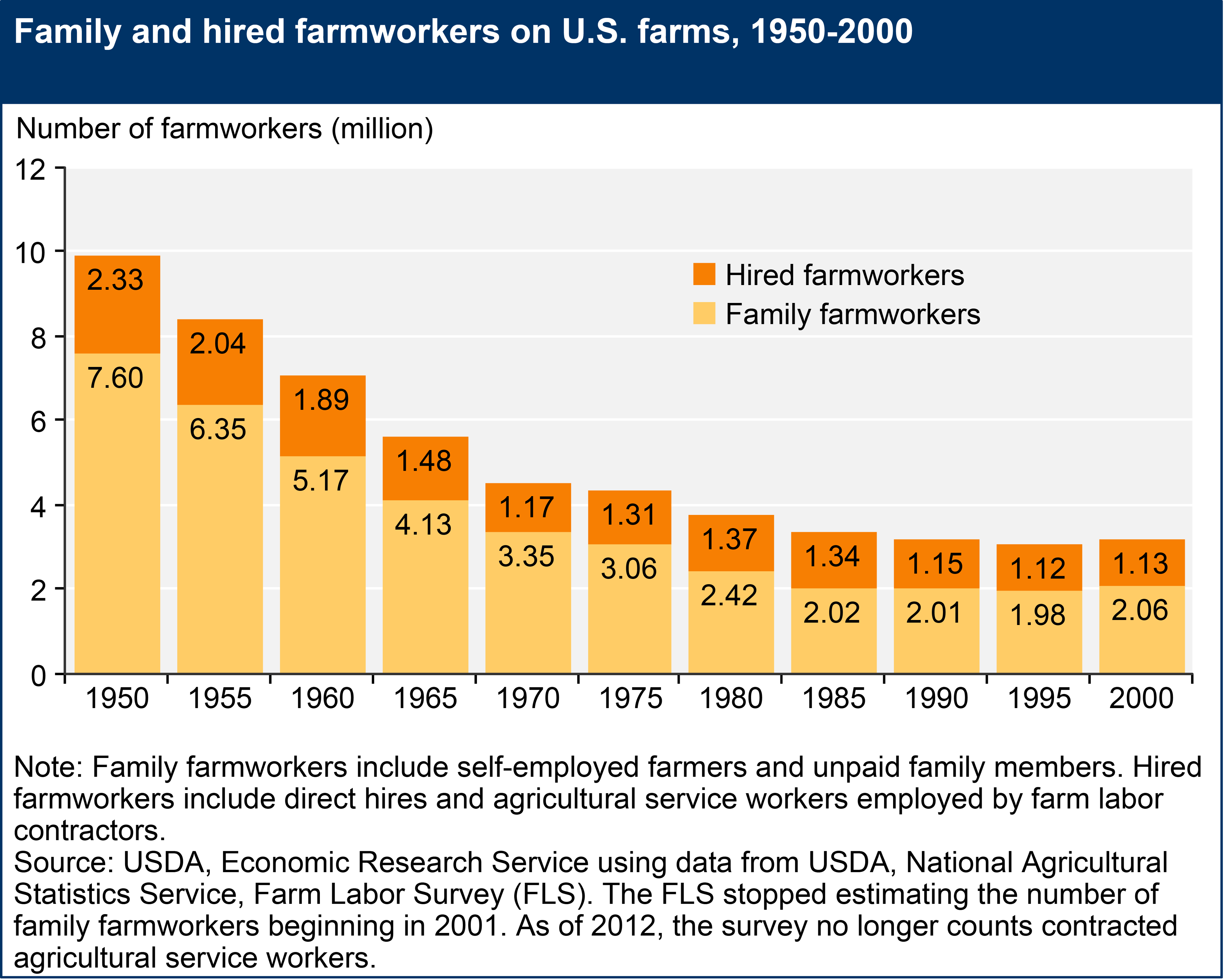
    The average number of hired farmworkers has steadily declined over the last 50 years, from roughly 2.33 million to just over 1 million (Figure 1).  Hired farmworkers make up less than 1 percent of all U.S. wage and salary workers, but they play an essential role in U.S. agriculture.  Labor expenses are a major concern for agricultural producers in general, but even more for fruits and vegetable producers.  Labor expenses for agricultural production accounts for around 10 percent of total operating expenses, however, labor expenses for fruits and vegetables are 38.5 percent and 28.8 percent, respectively.

    According to the U.S. Department of Labor’s National Agricultural Workers Survey (NAWS) estimates from data spanning fiscal years 2018–20, just 30 percent of crop farm workers in manual labor occupations were U.S. born, therefore around 70 percent were foreign-born.  Imported labor, primarily from Mexico, seems to be the major source of farm labor for fruits and vegetable production in the U.S.  However, the decline of farm workers from Mexico has caused U.S. farm labor shortages.  The main reasons for the decline are the sharp decline in the Mexican fertility rate, a significant expansion in rural education, and an increase in per-capita income, which is now close to $20,000 per year (adjusted for the cost of living). The good news for U.S. farmers is that there is a great deal of persistence in farm work. If a rural Mexican does farm work for one year, there is more than a 90 percent likelihood that he or she will do farm work the following year. The bad news is that a transition away from farm work is underway. The supply of agricultural workers will not disappear immediately, but U.S. agriculture can expect to see a gradual decline in the availability of Mexican farm workers over time.

    This decline in migration along with increasing the state minimum wage, and removal of overtime pay exemptions by some states appear to have increased U.S. farm labor costs.  The federal minimum hourly wage is $7.25 and has not increased since 2009, but some states set their minimum wage higher than the federal one. Also, the Raise the Wage Act of 2023, introduced in the U.S. House of Representatives and U.S. Senate on July 25, 2023, if approved would gradually raise the federal minimum wage to $ 17 an hour by 2028. Nevertheless, farm wages in the U.S. often exceed state minimum wages and are considerably higher than the Mexican minimum wage of $14 per day.

    Figure 1. Family and Hired Farmworkers on U.S. Farms, 1950-2000

    References

    Economic Research Service (ERS). “Farm Labor.” Accessed February 2024. https://www.ers.usda.gov/topics/farm-economy/farm-labor/. Updated August 7, 2023.

    Foreign Agricultural Service (FAS). Global Agricultural Trade System (GATS). Online database. https://apps.fas.usda.gov/gats/default.aspx. Online public database accessed February 2024.


    Ribera, Luis, and Landyn Young. “Challenges for U.S. Fruits and Vegetables.Southern Ag Today 4(28.4). July 11, 2024. Permalink