Blog

  • Digging into Dirt: Southern States Adoption of No-Till and Reduced Tillage Practices 

    Digging into Dirt: Southern States Adoption of No-Till and Reduced Tillage Practices 

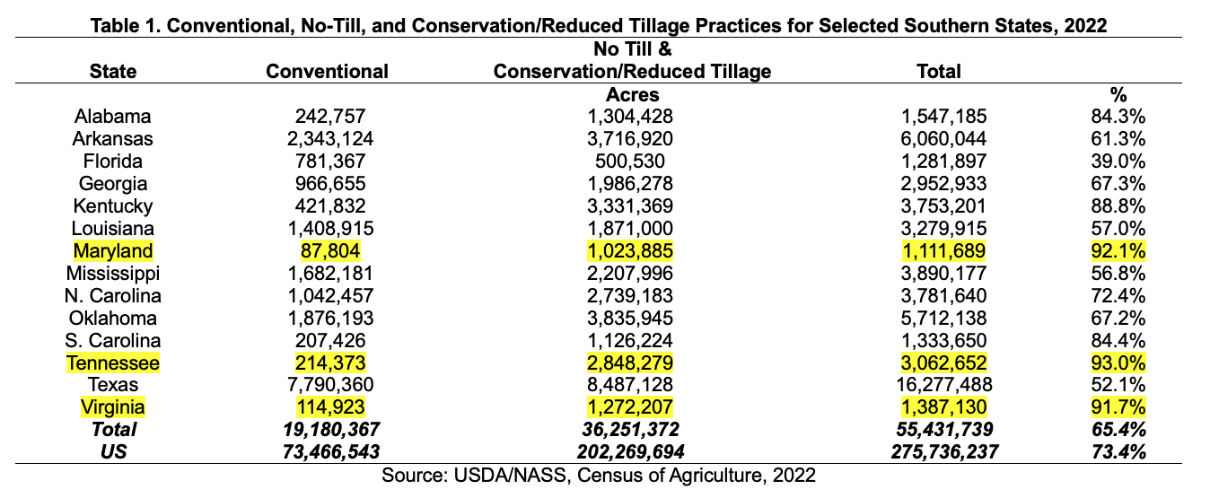
    Based on the USDA’s most recent Census of Agriculture 2022 data for tillage practices, no-till, and conservation/reduced tillage acres comprise 65.4% of the tillage practices for selected southern states (Table 1). For the US, the no-till and conservation/reduced tillage rate is 73.4%. No-till is defined as leaving 50% or more of the soil surface undisturbed from harvest to planting. Whereas conservation and reduced tillage is defined as leaving 30% or more surface undisturbed and may involve chisel plows or light disking (Rust and Williams, 2010). As of 2022, three southern states have the highest rate of no-till and conservation/reduced tillage in the U.S.: Tennessee (93%), Maryland (92.1%), and Virginia (91.7%). The three southern states with the smallest adoption of no-till and conservation/ reduced tillage practices compared to all tillage practices were Florida (39%), Texas (52.1%), and Mississippi (56.8%).

    Of interest would be the comparison of southern state’s adoption of these tillage practices over time, which are indicated in Figure 1. The figure displays the percentage change in no-till and conservation/reduced tillage acres at the county level from 2017 to 2022. Green shades indicate percentage decreases in these tillage practices whereas blue shades indicate an increase percentage wise.

    Figure 1. 2017 to 2022 Percentage Change in No-Till and Reduced/Conservation Tillage Acres

    Source: USDA/NASS Census of Agriculture, 2022

    The five southern states with the highest increase in acreage of cropland using no-till plus conservation/reduced tillage practices from 2017 to 2022 are Arkansas (17.6%), followed by Florida (15.3%), Texas (15.1%), Georgia (10.8%), and Alabama (10.7%). The states with the largest average increase in these tillage practices for the three census periods (2012, 2017, and 2022) were Florida (29.3%), Mississippi (20.6%), Arkansas (20.2%), Texas (17.1%), and Louisiana (16.4%).

    This information helps us understand which regions within the South are adopting reduced and no-till practices and is also relevant as carbon markets expand.  These practices can improve soil health by preserving soil structure, increasing water retention and organic matter. Additionally, they reduce soil erosion and lower greenhouse gas emissions by minimizing soil disturbance. However, given the cropping system, adopting no-till or reduced till may not make sense (e.g., peanut and rice production). Most importantly, the impact and profitability of no-till and reduced-till practices varies depending on the regions and crops involved, influencing adoption rates.

    Reference

    Rust, B. & J. Williams. 2010. USDA/ARS. “How Tillage Affects Soil Erosion and Runoff.” USDA/ARS Available at https://www.ars.usda.gov/ARSUserFiles/20740000/PublicResources/How%20Tillage% 20Affects%20Soil%20Erosion%20and%20Runoff.pdf.


    Menard, R. Jamey, and Hence Duncan. “Digging into Dirt: Southern States Adoption of No-Till and Reduced Tillage Practices.Southern Ag Today 4(31.3). July 31, 2024. Permalink

  • Cattle and Drought in the South and Southeast 

    Cattle and Drought in the South and Southeast 

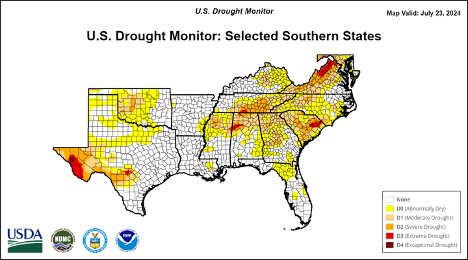
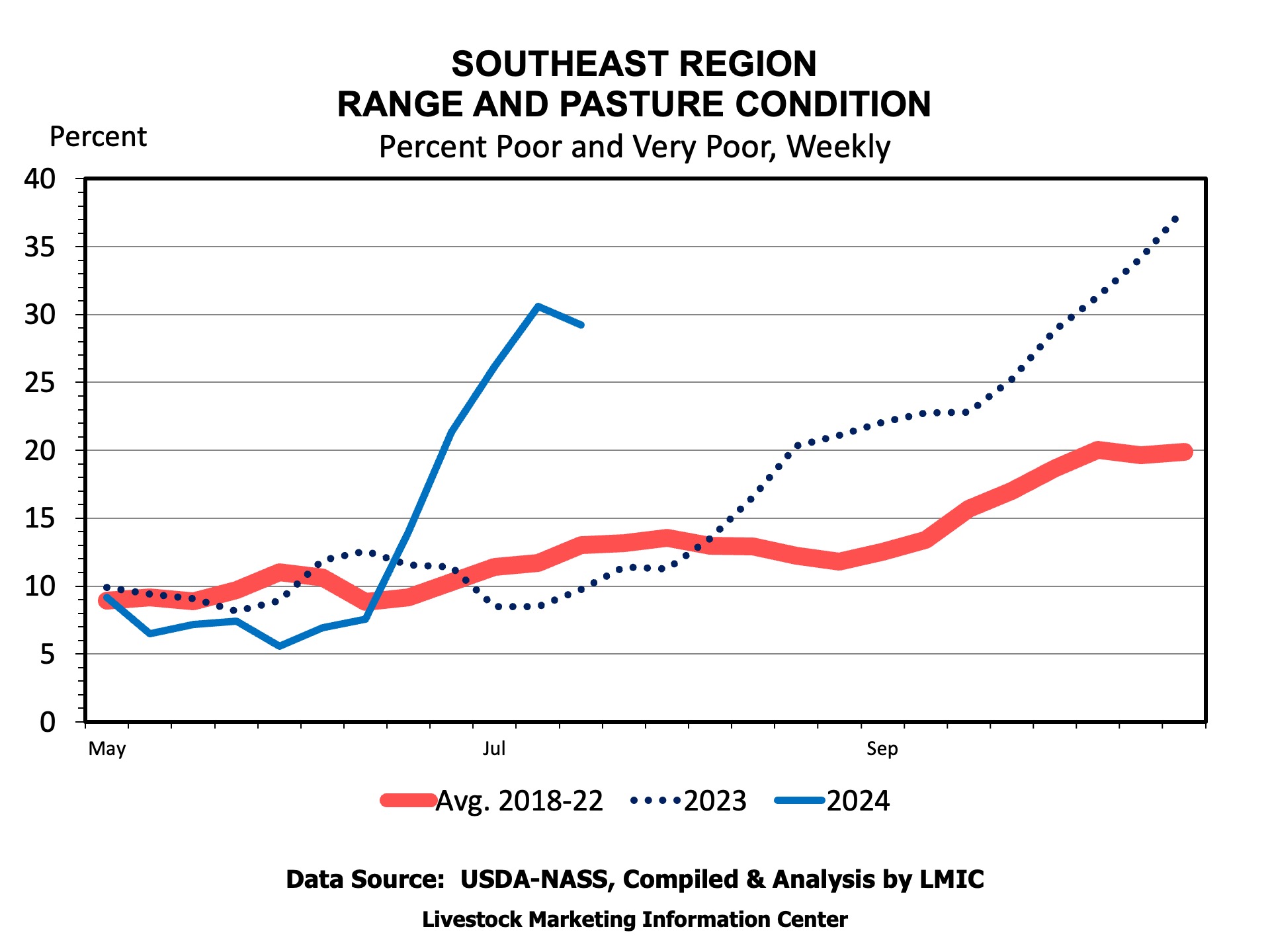
    Drought gripped the Southeast U.S. starting in June and has continued into July. More than 60 percent of the Southeast (AL, FL, GA, NC, SC, and VA) is experiencing drought. These drought conditions have hurt pasture and rangeland conditions in the Southeast. According to the USDA in mid-July, about 30 percent of the pasture in the Southeast (AL, AR, FL, GA, KY, LA, MS, NC, SC, TN, VA, WV) are in poor or very poor condition. Some drought conditions persist in other areas of the South, as well, including approximately half of Texas, 60 percent of Oklahoma, and 70 percent of Tennessee.

    Figure 1: Drought Conditions in the South

    Source: UNL Drought Monitor

    Should these drought conditions persist, producers will have several decisions to make related to feeding alternatives, forage management, marketing, and other areas. These decisions have implications for a host of different producer outcomes. Economics calls on producers to assess each decision along the following lines: How do revenues and costs change with each decision? This is the essence of a partial budget. A partial budget assesses the change in revenue and the change in costs associated with a change in practice. If changing practices increases net returns, you should change your practice. If not, continue with your baseline practice.Drought creates some uncertainty to the price outlook for this fall. If drought incentivizes producers to bring more calves to market compared to normal, while still remaining high compared to recent history, calf prices may see a more pronounced seasonal dip this fall. 

    Drought creates some uncertainty to the price outlook for this fall. If drought incentivizes producers to bring more calves to market compared to normal, while still remaining high compared to recent history, calf prices may see a more pronounced seasonal dip this fall. Timing may play a role, too. If calves are sold early, the fall low may be more spread out over time and not as deep. Lastly, if the weather improves, any expectations of more cattle this fall may evaporate pushing prices higher than expected. The next several weeks will be important in assessing where cattle markets will be in the months ahead.


    Secor, William. “Cattle and Drought in the South and Southeast.Southern Ag Today 4(31.2). July 30, 2024. Permalink

  • Review of 2023 STAX Payments and Implications for Price Risk Management in Cotton

    Review of 2023 STAX Payments and Implications for Price Risk Management in Cotton

    The USDA Risk Management Agency (RMA) published final 2023 county yields for upland cotton on July 3, 2024.  Upland cotton producers who purchased 2023 crop year Stacked Income Protection Plan (STAX) policies are now receiving final indemnity payments, thus contributing to current cash flow.  Based on RMA’s Summary of Business reporting as of July 15, total STAX indemnities across all states for 2023 will slightly exceed $352.7 million dollars.

    STAX is a crop insurance product for upland cotton that provides coverage for a portion of the expected revenue in an area. Most often, the “area” will be a specific county, but may include other counties or production practices as necessary to obtain a credible amount of data to establish an expected yield and premium rate. STAX coverage is available in all counties where crop insurance for upland cotton is currently offered.

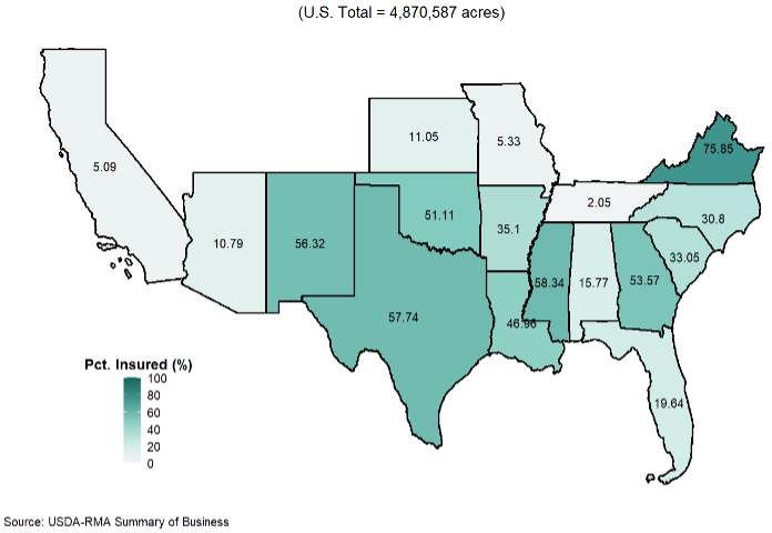
    According to USDA-RMA data, 4.87 million acres of upland cotton were insured under STAX in 2023 (Figure 1).  This was 48 percent of nearly 10.1 million planted acres.  In the majority of cotton producing states, STAX participation is much lower than 48 percent.  The high concentration of U.S. cotton acreage in Texas inflates the level of total participation in the STAX program.  On a regional basis, the Southwest (Kansas, Oklahoma, and Texas) accounted for 70 percent of the total acres enrolled in STAX last year.  This region also has the largest concentration of upland cotton acreage in the U.S at almost 6.1 million acres.  Texas alone planted over one-half or 5.55 million acres of the U.S. upland cotton total in 2023. Furthermore, Texas accounted for 66 percent, or 3.2 million of the 4.87 million total acres insured under STAX. 

    Figure 1. State-Level Percentage of Upland Cotton Planted Acres Enrolled in STAX (2023)

    STAX pays a loss on an area-wide basis, and an indemnity is triggered when there is an area loss in gross revenue. Gross revenue is a function of both yield and price.  Common to many crop insurance products, STAX utilizes a futures price (i.e. December cotton futures) to determine the Projected and Harvest prices used to calculate indemnity payments.  For most states in 2023, revenue losses resulted solely from below-average yields, which means that Projected and Harvest prices in those states were either the same or Harvest prices were higher than Projected prices.  

    The state level price discovery periods and the 2023 Projected and Harvest prices for cotton are summarized in Table 1.  Only Kansas, New Mexico and Oklahoma had a lower Harvest Price that may have contributed to revenue losses. Thus, for fourteen (14) of the seventeen (17) cotton producing states, any STAX payments were the result of actual yields being at least 10 percent less than the expected county/area yield (assuming the 90 percent area loss trigger was selected).

    Table 1. State Level Crop Insurance Price Discovery Periods for Cotton.

    State(s)Projected Price Discovery PeriodHarvest Price Discovery Period2023 Projected Price/lb2023 Harvest Price/lb
    Southern TX12/15 – 1/149/1 – 9/31$0.81$0.87
    AL, AZ, AR, CA, FL, GA, LA, MS, NC, SC, central TX1/15 – 2/1410/1 – 10/31$0.85$0.85
    MO, northern TX, TN, VA2/1 – 2/2810/1 – 10/31$0.84$0.85
    KS, NM, OK2/1 – 2/2811/1 – 11/30$0.84$0.78
    Source: USDA, Risk Management Agency

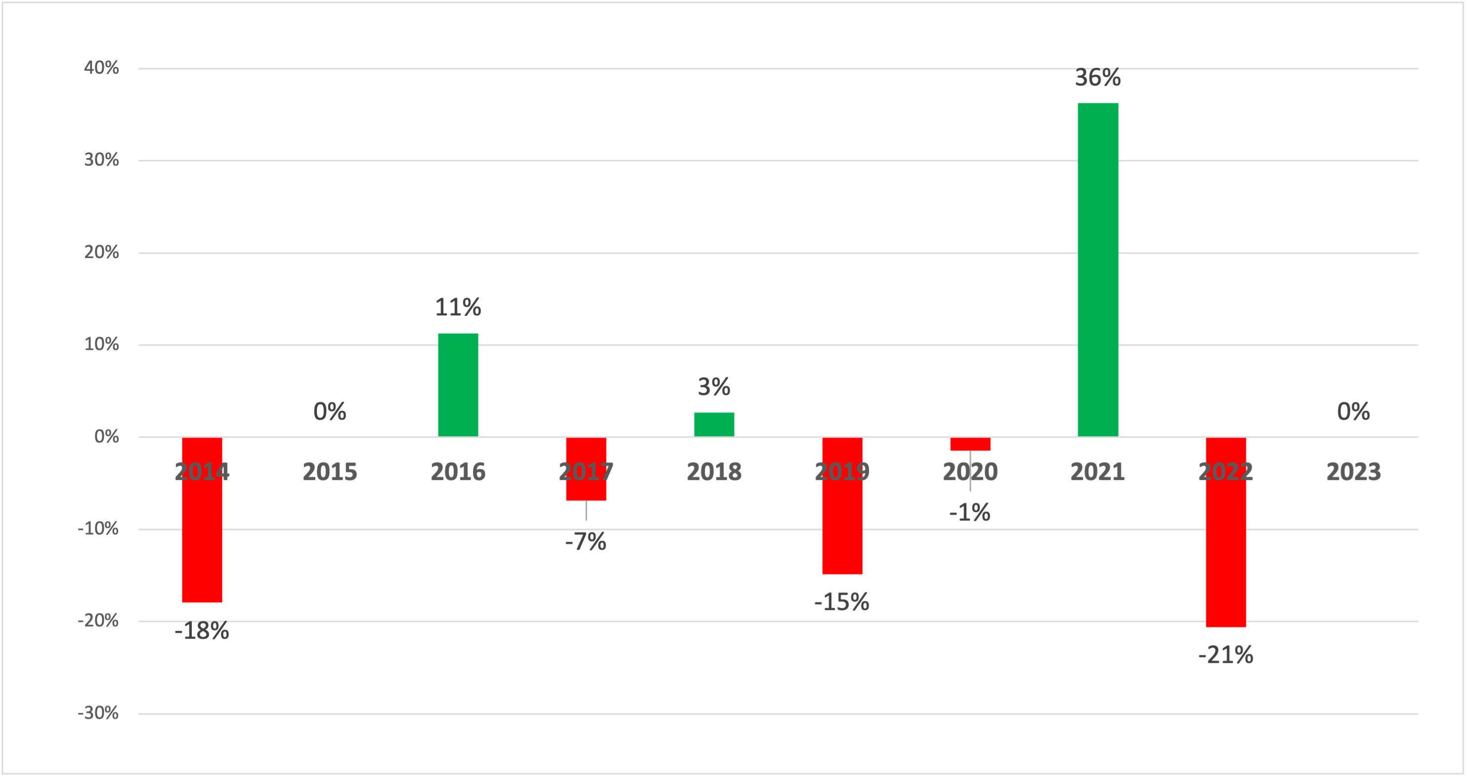
    Since the inception of the STAX program ten years ago, in response to the provisions in the 2014 Farm Bill, some consideration can be given to how effective the product is as a price risk management tool.  Although coverage levels can vary, the majority of STAX policies in the U.S. would see indemnities begin when area revenue falls below 90% of its expected level.  In selecting a crop insurance product, growers may consider the likelihood of a STAX revenue loss being generated solely by declining prices.  Figure 2 illustrates that over the past decade Harvest Prices relative to Projected Prices have experienced a 10 percent or greater decline in three crop years in the period 2014 to 2023, with an average change of -1.2%. Thus, similar to 2023, STAX most often protects against either only yield effects or a combined yield and price effect.  

    Figure 2. Percent Price Change from Projected to Harvest Price*, December Cotton Futures (2014 – 2023)

    Source: USDA, Risk Management Agency.
    *Price discovery periods for: AL, AZ, AR, CA, FL, GA, LA, MS, NC, SC, central TX.

    References

    USDA-RMA (2024, July). USDA Risk Management Agency Summary of Business. 

    URL: https://www.rma.usda.gov/SummaryOfBusiness.

    USDA-RMA (2024, July). USDA National Agricultural Statistics Service QuickStats. 

    URL: https://quickstats.nass.usda.gov/.


    Stiles, H. Scott, and Hunter D.Biram. “Review of 2023 STAX Payments and Implications for Price Risk Management in Cotton.Southern Ag Today 4(31.1). July 29, 2024. Permalink

  • In Landmark Ruling SCOTUS Overturns ‘Chevron’ Deference

    In Landmark Ruling SCOTUS Overturns ‘Chevron’ Deference

    On June 28, 2024, the United States Supreme Court issued its highly anticipated decision in Loper Bright Enters. v. Raimondo, No. 22-451 (2024). The case focused on the question of federal agency authority, and asked the Court to revisit its decision in the 40-year-old Chevron U.S.A., Inc. v. Natural Resources Defense Council, Inc., 467 U.S. 837 (1984) which famously established a legal test for judges to use when deciding whether a federal agency had acted outside its statutory authority. In a 6-3 decision, the Supreme Court officially overturned Chevron U.S.A., Inc. v. Natural Resources Defense Council, Inc., ruling that “courts may not defer to an agency interpretation of the law simply because a statute is ambiguous[.]”

    Chevron deference is a legal doctrine established by the Supreme Court to help courts determine when a judge should defer to a federal agency’s statutory interpretation. To apply Chevron deference, courts follow a two-step framework. First, the court should consider “whether Congress has directly spoken to the precise question at issue.” To make that determination, the court will review the relevant statute to see whether the language clearly addresses the issue targeted by the agency’s regulation or whether the statutory language is “ambiguous.” 

    If a court finds that the language is ambiguous, it will proceed to step two which requires the court to determine whether the agency’s statutory interpretation is “reasonable.” If the court finds that the interpretation is reasonable, then it must defer to the agency even if the court would have adopted a different interpretation. If the court concludes that the agency’s interpretation is not reasonable, then it may overturn the agency’s regulation. 

    In the decades since Chevron U.S.A., Inc. v. Natural Resources Defense Council, Inc. was first decided, it has become highly controversial. While some view Chevron deference as another tool of judicial interpretation, others regard it as a limitation on judicial authority.  

    At the Supreme Court, the plaintiffs in Loper Bright Enters. v. Raimondo challenged the doctrine of Chevron deference, specifically asking the Court to either overrule the doctrine or clarify its scope. In a majority ruling authored by Chief Justice Roberts, the Supreme Court overruled the doctrine, finding that the Administrative Procedure Act (“APA”) requires courts to “exercise their independent judgment” when determining whether an agency has acted outside of its statutory authority, and that “courts may not defer to an agency interpretation of the law simply because a statute is ambiguous[.]” The majority relied on past Supreme Court cases that address the role of courts and federal agencies in statutory interpretation, and the APA to reach its conclusion.

    In overturning Chevron U.S.A., Inc. v. Natural Resources Defense Council, Inc., the Supreme Court began by noting that Article III of the United States Constitution assigns to the federal judiciary the responsibility to hear and decide all “cases” and “controversies.” The Court then cited the foundational Supreme Court opinion, Marbury v. Madison, 5 U.S. (1 Cranch) 137 (1803). In that early case, which is regarded as establishing the scope of judicial review, the Supreme Court held that it is “the province and duty of the judicial department to say what the law is.” 

     Next, the Court reviewed its pre-Chevron case law on agency deference. The Supreme Court cited United States v. Moore, 95 U.S. 760 (1878) which explains that courts should give “the most respectful consideration” to federal agency interpretations of statutes they are tasked with administering because employees of such agencies are considered “masters of the subject[.]” The Court also cited Skidmore v. Swift & Co., 323 U.S. 134 (1944), where the Supreme Court held that a federal agency’s statutory interpretations “constitute a body of experience and informed judgement to which courts and litigants [could] properly resort for guidance,” but that such interpretations would not control a reviewing court’s own statutory interpretations.  After reviewing these cases, the majority concluded that prior to its ruling in Chevron U.S.A., Inc. v. Natural Resources Defense Council, Inc., the Supreme Court had consistently held that while a federal agency’s statutory interpretations could be given due respect by a reviewing court, it was ultimately up to the judiciary to determine the proper meaning of the law.

    Along with reviewing its own case law, the Supreme Court also examined the text of the APA. The APA is the federal law that governs the way federal administrative agencies develop regulations, and  establishes standards for judicial review of agency actions.  The law states that “[t]o the extent necessary to decision and when presented, the reviewing court shall decide all relevant questions of law, interpret constitutional and statutory provisions, and determine the meaning or applicability of the terms of an agency action.” 5 U.S.C. § 706. According to the Court, that statutory language represents Congress’s intent to have reviewing courts, not agencies, “decide all relevant questions of law” and “interpret […] statutory provisions.” The Court concluded that the Chevron doctrine cannot be reconciled with the APA because Chevron deference requires courts to adopt reasonable agency interpretations of statutory language, even if the court would have reached a different interpretation. According to the majority, this does not comply with the APA’s requirement that courts “shall decide all relevant questions of law.”

    Based on its review of both previous Supreme Court decisions, and the text of the APA, the majority in Loper Bright Enters. v. Raimondo concluded that “[i]n an agency case as in any other […] there is a best reading [of the law] all the same – ‘the reading the court would have reached’ if no agency were involved.” Following this ruling, when a court is presented with a case that involves statutory interpretation, it may not “defer to an agency interpretation of the law simply because a statute is ambiguous.” Instead, it is the role of the court to apply its own judgement to determine what the law says.


    Rollins, Bridgit. “In Landmark Ruling SCOTUS Overturns ‘Chevron’ Deference.Southern Ag Today 4(30.5). July 26, 2024. Permalink

  • Understanding the Growing U.S. Agricultural Trade Deficit (Part 2): What’s Happening with Imports?

    Understanding the Growing U.S. Agricultural Trade Deficit (Part 2): What’s Happening with Imports?

    A trade deficit occurs when the value of a country’s imports exceeds its exports. Although we often refer to the overall trade deficit (all goods), there is a growing concern about the rising U.S.  agricultural trade deficit. Recall that the most recent trade outlook report published in May 2024 by the Economic Research Service and Foreign Agricultural Service – agencies of the U.S. Department of Agriculture (USDA) – projected the highest agricultural trade deficit to date in fiscal year (FY) 2024 (October 2023 – September 2024). The FY2024 forecast have has U.S. agricultural exports at $170.5 billion, but imports at $202.5 billion. If these projections hold true, the resulting agricultural trade deficit would be a record $32 billion. To put this in context, U.S. agricultural exports have far exceeded imports in past years. It is only in recent years that U.S. agricultural trade became more balanced. FY2023 was the first year the U.S. experience a significant agricultural trade deficit ($16.7 billion), which is half the projected deficit for FY2024 (Kaufman et al., 2024). In a previous Southern Ag Today article we discussed how declining agricultural exports have contributed to the growing U.S. agricultural trade deficit. In this article we discuss the contribution of rising agricultural imports.

    U.S. agricultural imports are very different from exports. U.S. agricultural exports are dominated by bulk commodities like soybeans, corn, cotton and wheat, and minimally processed products like tree nuts, beef, and pork. Even though value added products like dairy products and prepared foods are also among top U.S. agricultural exports, U.S. agricultural imports are overwhelmingly higher value consumer-oriented products. In 2023, for instance, the major U.S. imports included fresh fruits ($18 billion), other vegetable oils ($13 billion), fresh vegetables ($12 billion), distilled spirits ($11 billion), beef products ($9 billion), coffee ($9 billion), soup and other prepared food ($7 billion), wine ($7 billion), and beer ($7 billion). Other than beef and maybe prepared foods, imports of these products greatly exceed their exports. For instance, U.S. imports of beer, wine, and spirits were around $25 billion in 2023, whereas U.S. beer, wine, and spirit exports were less than $4 billion (USDA, 2024).

    Figure 1 shows the unit values for U.S. agricultural imports and exports from 2010-2023. On a per-unit basis ($/MT), U.S. imports are significantly more expensive than exports. Since 2010, imports have been two to three times more expensive. In 2023, the import unit value was $2,543/MT versus $919/MT for exports. U.S. agricultural exports were almost 190 million MT in 2023, while imports were only 77 million MT. However, imports were valued at $196 billion, while exports were valued at $174 billion. When considering the period where the U.S. experienced significant price inflation (2020–2022), import prices increased at a much higher rate that export prices, which is to be expected given that imports are made up of higher value consumer goods. During this period, the quantity of imports continued to increase despite rising prices, but the quantity of exports declined. The main takeaways from this article are the following. 1) U.S. agricultural imports are very different than exports; 2) imports are significantly more expensive and more subject to inflationary pressures than exports; and 3) imports have persistently risen despite rising prices in recent years, which was not the case for U.S. agricultural exports.

    Figure 1. Import and Export Prices: 2010 – 2023

    Source: U.S. Department of Agriculture (USDA, 2024).

    For more information

    Kaufman, James, Hui Jiang, Bart Kenner, Angelica Williams, and Adam Gerval. (2024). Outlook for U.S. Agricultural Trade: May 2024. Report AES-128. U.S. Department of Agriculture. https://www.ers.usda.gov/publications/pub-details/?pubid=109252

    U.S. Department of Agriculture (USDA). 2024. Global Agricultural Trade System (GATS). Foreign Agricultural Service. https://apps.fas.usda.gov/gats/default.aspx


    Muhammad, Andrew, and Md Deluair Hossen. “Understanding the Growing U.S. Agricultural Trade Deficit (Part 2): What is Happening with Imports?Southern Ag Today 4(30.4). July 25, 2024. Permalink