Blog

Reference Prices: Setting the Record Straight
With cotton added back to the farm safety net via the Bipartisan Budget Act of 2018, the 2018 Farm Bill largely maintained the statutory reference prices (SRPs) established in the 2014 Farm Bill. One noticeable exception was the addition of Effective Reference Prices (ERPs) in the 2018 Farm Bill at the insistence of House Republican negotiators. As we noted in a December 2022 Southern Ag Today article, Section 1101 of the 2018 Farm Bill (P.L. 115-334) allows for the ERP for a commodity to replace the SRP if 85% of the previous five-year Olympic average of the national marketing year average price is greater than the SRP. The ERP may increase to as much as 115% of the SRP.

A recent article noted that the Congressional Budget Office (CBO) is projecting that “9 of the 19 program crops will have an ERP higher than the SRP in at least some of the years of the baseline” with those crops representing “over 90% of all base acres in the United States.” They argue that this will result in an increase in Reference Prices “without Congress needing to do anything more than extend those [ERP] provisions.” While the article expressed surprise at “how little attention the ERP has received,” we have been reporting on it since the inception of Southern Ag Today as noted above. It seems the real purpose of this new article was to call into question the need for higher SRPs in the next farm bill, a key request of many state and national commodity organizations across the country. We believe this latest article seriously misses the mark in two key respects:
- First, while there is no question that the ERP provision is projected to result in higher Reference Prices for certain crops, it is projected to have zero impact on several other major commodities, including cotton, rice, and peanuts. While the author acknowledged this point, he simply used the absence of an increase in market prices for these other crops as a nonsensical justification for not adjusting the SRPs for these crops. As we’ve noted elsewhere (including in recent Southern Ag Today articles), sticky production costs and the prospect of lower prices are the primary justifications for increased SRPs (frankly, for all covered commodities).
- Second, while ERPs are certainly projected to provide higher levels of protection for some crops, those levels will also drop if marketing year average prices fall going forward. As a result, while CBO’s relatively flat price projections are an important factor in the debate, the much more important consideration for policymakers is how the farm safety net will fare if those projections are wrong. To that end, we analyzed the impact of an unforeseen price drop on all 64 crop farms maintained by the Agricultural & Food Policy Center (AFPC) at Texas A&M University. Specifically, we examined the impact of a price decrease over the next 5 years assuming that crop prices followed the same path experienced during the last downturn from 2013 to 2017. Under this scenario, 33 of the 64 crop farms maintained by AFPC would face a greater than 50% likelihood of an ending cash shortfall at the end of the baseline outlook (2028). In other words, under that scenario, 52% of the farms would have a greater than 50% chance of exhausting all cash on hand over the next 5 years and would have to debt-finance the day-to-day operations of the farm. Bottom line: if there are any unforeseen hiccups in the market, the current farm safety net is simply NOT up to the task of mitigating losses for many farms across the country.
As we’ve noted time and again, the farm bill debate is fertile ground for those who like to sow regional discord. Serious observers know that the farm bill must work for growers throughout the United States and not just one region of the country. If the goal is to ensure that the farm safety net can provide meaningful levels of support for producers in the event of a downturn in the farm economy, simply relying on existing Effective Reference Prices – or even modest 5-10% increases in the Statutory Reference Prices for many covered commodities – will simply prove insufficient. Producers are operating in a higher cost environment, the Federal farm safety net needs to reflect that fact. We are all for the swift completion of the farm bill, but given the extraordinary amount of capital that American producers are putting at risk, we continue to believe that the substance of the farm bill is far more important than the timeline.

Fischer, Bart L., and Joe Outlaw. “Reference Prices: Setting the Record Straight.“ Southern Ag Today 3(41.4). October 12, 2023. Permalink
October 12, 2023

Capital Recovery Costs: An Important Component of Enterprise Budgeting

Although it is early in the harvest season for many crops grown in the South, it is time to begin revising your annual enterprise budgets in preparation for the 2024 growing season. Enterprise budgets are forward-looking estimates of production costs on a per acre basis for a particular enterprise and production method (e.g, cotton on non-irrigated land).

When it comes to enterprise budgets, direct operating costs are straightforward. If a grower plans to use an input, they specify the amount they plan to use per acre and multiply that by the price per unit of that input. The product is an estimate of the operating cost per acre to charge to that enterprise.

Some overhead costs, also known as ownership costs, are more complex because they are noncash expenses. One may wonder why it is important to charge noncash expenses to an enterprise. There are two reasons for this. First, the use of owned equipment causes wear and tear over time. Eventually, owned equipment needs to be replaced. The loss in value overtime, or depreciation, should be charged to the enterprise for the use of that equipment. Second, the capital invested in the equipment could be invested elsewhere and earn a percentage return on that investment. This opportunity cost, or interest expense, should also be charged to the enterprise.

One effective method of calculating these noncash overhead costs is using the capital recovery method. The capital recovery method enables growers to estimate an annual per acre cost in present day dollars based on the useful life of the equipment used by the enterprise. The following equation can be used to calculate annual capital recovery cost per acre.

-where n represents the useful life of the equipment and i represents the interest rate. The table below lists capital recovery factors (CRF) by year (n) and interest rate (i).

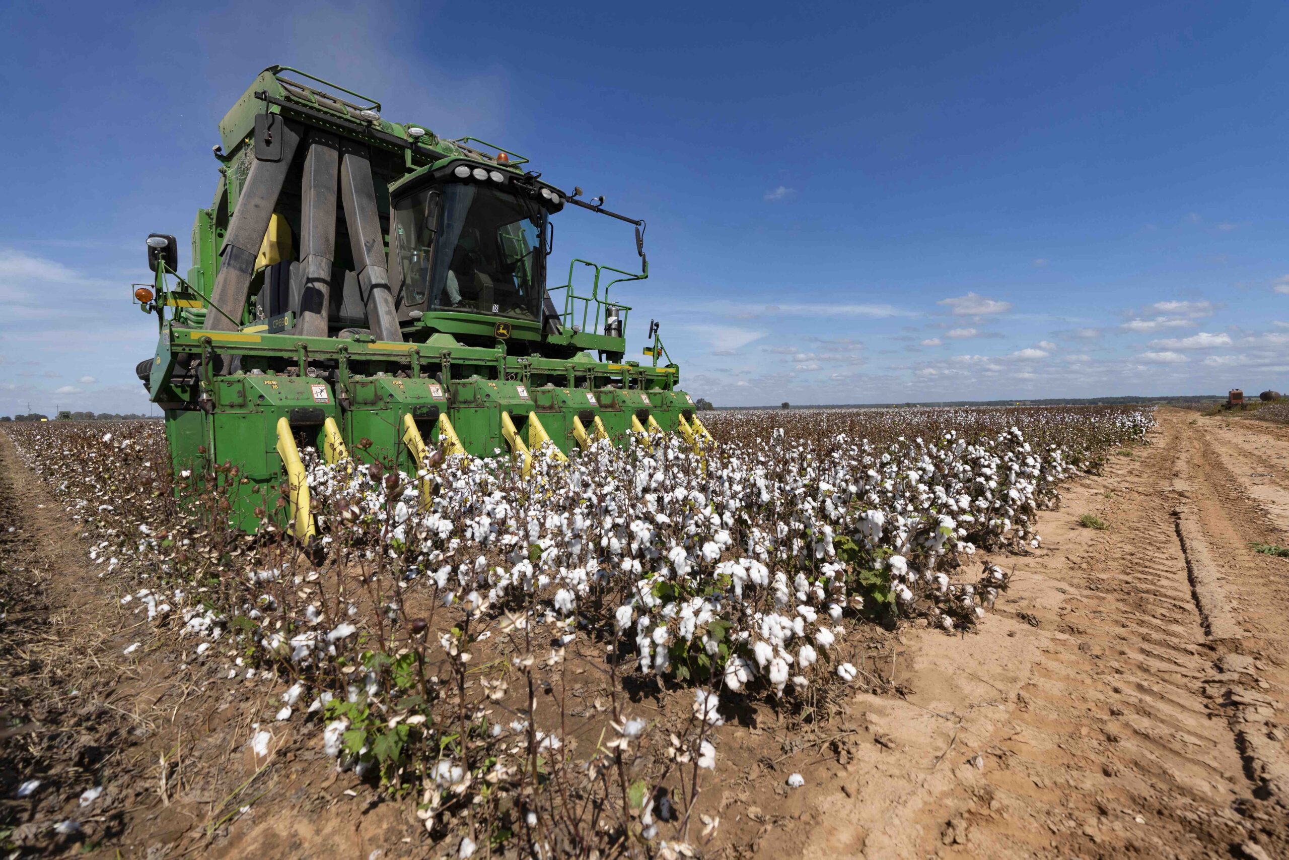
Some row crops are more capital-intensive than others because they require commodity-specific harvest equipment. This is certainly the case for cotton and peanuts in the South. Grain growers need one combine to harvest their grain, and different headers can be switched out to harvest corn, soybeans, and wheat/other small grains. Cotton farmers need a cotton picker or stripper to harvest cotton, and it cannot be used to harvest any other crop. Peanut farmers need a digger/inverter to dig and invert peanut vines and then use a peanut picker to pick the peanuts off the vines. Like cotton, peanut harvest equipment cannot be used to harvest any other crop.

Figure 1 provides an example of annual capital recovery cost per acre at different interest rates for cotton, peanut, and grain harvesting equipment. The appropriate interest rate to select depends upon the grower, their risk tolerance, and desired rate of return on their investments. The average range is between 8-10%, with 9% highlighted on the chart.

The harvest equipment used in this example are based on typical equipment sizes used in Georgia (6-row equipment on 36-inch row spacing) and are assumed to be new. Capital recovery costs can also be calculated on used equipment based on the equation above. Table 1 lists the assumptions on purchase price, salvage value, useful life, and total annual harvest acres. Note, since the harvest equipment is only being evaluated in this article, the tractor has similar total acres to the sum of the peanut digging and picking quipment which are pulled by the tractor, with some allowance for turnaround at the end of the rows. The grains combine is assumed to harvest multiple crops like corn and soybeans.

Table 1 Title: Assumptions on purchase price, salvage value, useful life, and total annual harvest acres.

Figure 1 Title: Sensitivity Analysis of the Annual Capital Recovery Cost per Acre for Cotton, Peanut, and Grains Harvest Equipment.

Chart Source: Author created, using a capital recovery factor table, data on purchase prices, and assumptions on salvage value, useful life, and annual use.

It is evident that cotton and peanuts are more capital-intensive because of the specific harvest equipment and those enterprise budgets need to account for those higher costs per acre. Furthermore, interest rates matter. As interest rates increase, capital recovery costs do too.

While this is only an example for harvesting equipment, this method should be used for each machine used in producing a specific enterprise and added together to determine the total annual capital recovery cost. Table 2 lists a range of capital recovery factors by year and interest rate to aid growers in tabulating these costs on all of their equipment owned by the farm.

Table 2 Title: Capital Recovery Factors (CRF) by Year (n) and Interest Rate (i)

Useful Life(Years)	2.0%	3.0%	4.0%	5.0%	6.0%	7.0%	8.0%	9.0%	10.0%	11.0%	12.0%	13.0%	14.0%	15.0%
Useful Life(Years)
1	1.020	1.030	1.040	1.050	1.060	1.070	1.080	1.090	1.100	1.110	1.120	1.130	1.040	1.150
2	0.515	0.523	0.530	0.538	0.545	0.553	0.561	0.568	0.576	0.584	0.592	0.599	0.607	0.615
3	0.347	0.354	0.360	0.367	0.374	0.381	0.388	0.395	0.402	0.409	0.416	0.424	0.431	0.438
4	0.263	0.269	0.275	0.282	0.289	0.295	0.302	0.309	0.315	0.322	0.329	0.336	0.343	0.350
5	0.212	0.218	0.225	0.231	0.237	0.244	0.250	0.257	0.264	0.271	0.277	0.284	0.291	0.298
6	0.179	0.185	0.191	0.197	0.203	0.210	0.216	0.223	0.230	0.236	0.243	0.250	0.257	0.264
7	0.155	0.161	0.167	0.173	0.179	0.186	0.192	0.199	0.205	0.212	0.219	0.226	0.233	0.240
8	0.137	0.142	0.149	0.155	0.161	0.167	0.174	0.181	0.187	0.194	0.201	0.208	0.216	0.223
9	0.123	0.128	0.134	0.141	0.147	0.153	0.160	0.167	0.174	0.181	0.188	0.195	0.202	0.210
10	0.111	0.117	0.123	0.130	0.136	0.142	0.149	0.156	0.163	0.170	0.177	0.184	0.192	0.199
11	0.102	0.108	0.114	0.120	0.127	0.133	0.140	0.147	0.154	0.161	0.168	0.176	0.183	0.191
12	0.095	0.100	0.107	0.113	0.119	0.126	0.133	0.140	0.147	0.154	0.161	0.169	0.177	0.184
13	0.088	0.094	0.100	0.106	0.113	0.120	0.127	0.134	0.141	0.148	0.156	0.163	0.171	0.179
14	0.083	0.089	0.095	0.101	0.108	0.114	0.121	0.128	0.136	0.143	0.151	0.159	0.167	0.175
15	0.078	0.084	0.090	0.090	0.096	0.103	0.117	0.124	0.131	0.139	0.147	0.155	0.163	0.171
16	0.074	0.080	0.086	0.092	0.099	0.106	0.113	0.120	0.128	0.136	0.143	0.151	0.160	0.168
17	0.070	0.076	0.082	0.089	0.095	0.102	0.110	0.117	0.125	0.132	0.140	0.149	0.157	0.165
18	0.067	0.073	0.079	0.086	0.092	0.099	0.107	0.114	0.122	0.130	0.138	0.146	0.155	0.163
19	0.064	0.070	0.076	0.083	0.090	0.097	0.104	0.101	0.120	0.128	0.136	0.144	0.153	0.161
20	0.061	0.067	0.074	0.080	0.087	0.094	0.102	0.110	0.117	0.126	0.134	0.142	0.151	0.160

Smith, Amanda R. “Capital Recovery Costs: An Important Component of Enterprise Budgeting.” Southern Ag Today 3(41.3). October 11, 2023. Permalink

October 11, 2023

Cow Culling Climbing Seasonally

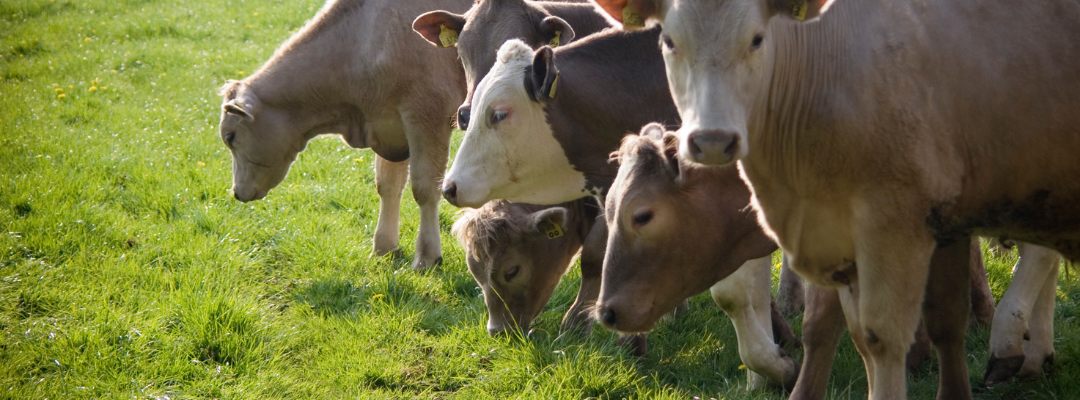
Cow culling, as indicated by the weekly cow slaughter data, is starting to increase going into the last quarter of the year but cow slaughter normally peaks in the Fall because that’s when more beef cow culling decisions are made.  For the week ending September 23^rd, the last data available, 127,600 cows went to federally inspected plants, the largest week since the last week of June.  For the year, cow slaughter has totaled 4.8 million head, 5.6 percent less than last year.

The total cow slaughter data masks the different seasonal patterns for beef cows and dairy cows.  Beef cow slaughter typically peaks in the Fall and is at its lowest around February-March.  Beef cow slaughter is down 13.4 percent compared to a year ago.  The data is reported by region with Region 6 including Texas, Oklahoma, Louisiana, and Arkansas.  The rest of the South (except Virginia) are reported in Region 4.  Beef cow slaughter in Regions 4 and 6 are 4.9 and 19.3 percent lower than last year, respectively.  Cow culling in the deep South has not fallen as much as the average across the country, while slaughter in the western part of the South has fallen faster than the average.  That may suggest some ability or willingness to try to expand herds in different parts of the region.

Dairy cow slaughter typically peaks in the January-March period.  Low milk prices and margins have triggered more culling this year with dairy cow slaughter 4.6 percent higher than last year.  Higher prices and improving margins over the last 3 weeks have finally pulled down dairy slaughter below a year ago.

Cull cow prices appear to have topped out seasonally and are starting to decline.  Southern Plains auction prices declined to $72 per cwt last week, their lowest since June.  While tight beef supplies are keeping prices high, the cull market loses the impact of grilling season demand once we are past Labor Day.

What to Watch For?

Even though beef cow culling normally increases this time of the year, watch for weekly slaughter relative to last year and the 5-year average.  The opportunity to begin herd expansion may begin with a smaller Fall run of cows this year, maybe even with a couple of weeks below the 5-year average.  We most likely saw the biggest weekly beef cow slaughter of the year back in January.  On the dairy side, watch for slaughter to remain below the 5-year average in the coming weeks.  Have enough dairy cows been culled to support a path to profitable production?  Can some cows be profitably held over the winter to take advantage of seasonal price increases next year with the added bonus of improved weight and quality along with, maybe, a calf to sell too?

Anderson, David. “Cow Culling Climbing Seasonally.” Southern Ag Today 3(41.2). October 10, 2023. Permalink

October 10, 2023
Who’s Holding Global Soybean Stocks?

The size of global soybean stocks is an important factor in determining global soybean prices, but the quantity held by different countries and annual use are also relevant to the market. In the 2018/19 marketing year (during the U.S.-China trade war), the U.S held 22% of global stocks compared to China (16%), Brazil (29%), Argentina (25%), and the rest of the world (8%). Since then, China has more than doubled its share of global stocks, while the U.S. ending stock has dropped to the lowest level in eight years. At the end of the 2023/24 marketing year, the U.S. is projected to hold 5% of global soybean stocks compared to China (33%), Brazil (32%), Argentina (21%), and the rest of the world (9%). Even though U.S. ending stocks are projected to be tight for the current marketing year, global stocks are projected to be an all-time record (Figure 1).

Figure 1. Projected Global Soybean Ending Stocks, by Country, at the End of the United States Marketing Year, 2012/2013 to 2023/2024

This analysis can be taken one step further by incorporating usage. Days-on-hand can be used to estimate a country’s stocks relative to annual use (domestic consumption + exports). China is projected to have 120 days of soybeans on hand for the past and current marketing year (Table 1). World days-on-hand are projected at 114 days, the second highest in the past 12 years. Argentina’s soybean days-on-hand are projected to increase from a 10-year low of 159 days to a high of 197 days, by the end of the current marketing year. Due to the abundance of global stocks and the projected days-on-hand, it may be challenging for U.S. soybean exports to achieve the current USDA projection of 48.7 million metric tons (MT). This would result in increased U.S. ending stock. Additional factors such as exchange rates, discussed in a prior Southern Ag Today article, will also play an important role in U.S. exports and ending stocks.

Based on current USDA projections, further weakness in soybean futures prices seems likely, unless a weather disruption in South America leads to reductions in projected production. A bounce back in Argentina’s drought reduced production (projected production was halved by last year’s drought) seems likely and Brazil is forecast to produce another record crop. January 2024 soybean futures have already decreased $1.49/bu since the July 24, 2023, high of $14.41/bu. A key level of support for the January contract is $12.60/bu-$12.80/bu. If prices fall below $12.60/bu, it is possible that prices test the contract low of $11.41/bu from May 31, 2023. For producers concerned with a decline in futures prices for unpriced soybeans that will be held in storage, an $11.70 put option could be purchased for 6 cents. This is cheap protection based on the large amount of uncertainty in the current South American soybean production year.

Table 1. Soybean Days-on-Hand by Country, 2012/2013 to 2023/2024

References and Resources

Barchart.com. https://www.barchart.com/futures/grains?viewName=main

USDA September WASDE. https://www.usda.gov/oce/commodity/wasde/wasde0923.pdf

Smith, Aaron. “Who’s Holding Global Soybean Stocks?” Southern Ag Today 3(41.1). October 9, 2023. Permalink

October 9, 2023

How Much Can I Sell This For? Part III

As a continuation of the “How Much Can I Sell This For?” series, this article focused on evaluating market potential. Part I, Part II.

Producers may have different opportunities with CSAs, restaurants, farmers markets, wholesale markets, on-farm, and retail outlets. So how can these avenues be evaluated? It will likely look different depending on the producer. For risk management purposes, it is recommended to set up multiple marketing channels. If one market is lost, there are still opportunities to make sales and find buyers for all of your products.

Important questions to ask include:

How much product do I need to move?
What options are available to me?
What type of customers are in that market?
Am I charging a low, middle, or high price?
Are there additional costs to participating in that market?

Typically, there will be an inverse relationship between quantity of product versus price. Meaning if you have few products, you will need a higher price per item to offset cost. Conversely, having greater quantity means lower cost per item but greater number of sales to make. A successful producer who builds relationships with multiple buyers will utilize several outlets and tiered pricing to hit their sales targets. Your marketing mix may also look different over time as you adapt to changing market needs and preferences.

Here is an example of how to evaluate market potential. Assume there is $100.00 additional cost to participate in a farmers market each week. This may include a fee for the market, paying an employee to go to the market, and fuel for traveling to and from the location. That $100.00 would need to be covered by sales that week (or over the course of the season) for the market to be viable. Some weeks you may hit the target and other weeks you may not. If a market consistently failed to meet your goals, it may be time to look at other options.

If you were to charge average pricing for tomatoes ($1.25 per pound), what would be your breakeven for the market given this scenario? Recalling the examples shared in Tables 1 and 2 of our article titled “How Much Can I Sell This For? (Part II)”, the cost of production for tomatoes (at 38,000 lbs./acre) is $.31 cents per pound. Remember the $100.00 of marketing cost that needs to be covered. With the current scenario, $1.25 (sales price) – $.31 (cost of production) = $.94 per pound goes toward marketing (and hopefully ultimately profitability). Only when the $100.00 from marketing is covered does the business move into profitable sales. So, with the current cost of production and marketing expense you would need to sell roughly 106 lbs. of tomatoes for the market to be viable (see Table 1).

Table 1. Example: Evaluate Market Potential including Marketing Costs for Field-grown Tomatoes (one acre)

Total Production Costs:	$11,500	/ 38,000 lbs. expected yield = $.31 per lb.

Sales Price:			$1.25	per lb.
Total Production Costs (subtract):			$0.31	per lb.
			$0.94	per lb.

Marketing Cost:			$100.00
			/ $.94	per lb.
So, need to sell approximately 106				lbs.

Perhaps that sounds like a lot to sell, so you decide to raise the sales price to $2.00/lb. Perhaps you determine the marketing cost is simply too high and it would be hard to recoup the cost. Perhaps you have three other vegetables you are selling and so the $100.00 is spread over additional items. This example looks at one product and one week at the market, but we know the season is longer and there are other markets and decisions you can make over that time period. If your price is high, you may have to adjust or find other markets. If your price is low, you may be hurting your bottom line and bringing down the overall prices others may charge in your market. Some markets have little to no marketing costs while others may charge a substantial amount. While it may be profitable, you may need to move higher volumes, so you decide to combine the farmers market and other market channels to move all your product. The analysis may be done with multiple variations, and the same principles apply but the process can become more complex with more variables present. The decision to market your own products presents additional challenges beyond agriculture production decisions, and these factors can change during the season.

To compete in the world of agribusiness often requires flexibility. Entering the market with a base level of knowledge provides information for you to be able to make informed decisions. Finding a particular crop or market is not viable can sometimes happen on paper before it becomes a reality. Additionally, being able to pivot and negotiate, because of your level of knowledge, is a business advantage. We hope this discussion has been useful as you think of your own goals and plans for profitability on your farm.

Burkett, Kevin. “How Much Can I Sell This For? Part III.” Southern Ag Today 3(40.5). October 6, 2023. Permalink

October 6, 2023

Blog

Reference Prices: Setting the Record Straight

Capital Recovery Costs: An Important Component of Enterprise Budgeting

Cow Culling Climbing Seasonally

Who’s Holding Global Soybean Stocks?

How Much Can I Sell This For? Part III