Blog

  • Beef x Dairy Placements

    Beef x Dairy Placements

    Over the last few years, there has been a lot of discussion/questions surrounding the impact of Beef x Dairy (BxD) on the beef supply chain. Anecdotally, BxD calves have gone from day olds being worth $75/head in 2019, to well over $800/head today. Thus, BxD calves have led to increased revenue for dairy producers around the country. Given their worth, dairy producers have increased the amount of BxD offspring in their breeding program. The increase has been noticed by the beef industry and has led to the particular question, “How many head of Beef x Dairy calves are out there?”. This is a common question that has been asked at Extension meetings, and most recently, at the 2025 Beef Improvement Federation (BIF) in Amarillo, TX. While it may seem simple to answer, it is quite difficult to answer that simple question. 

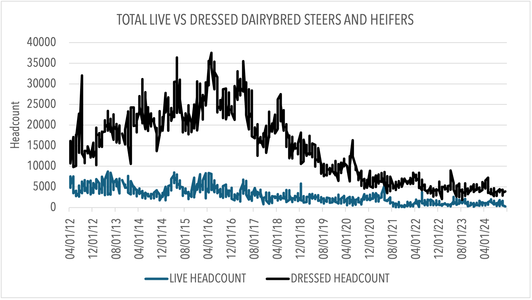
    Historically (from 2001-2024), the dairy herd size has remained relatively constant at 9.2 million head. Annually, the dairy calf crop is utilized as either future replacement heifers, or they enter the beef supply chain. The ones that enter the beef supply chain are eventually harvested and marketed as fed cattle. The cattle that are straightbred dairy (majority dairy genetics) are reported by the USDA as “dairy” in the fed cattle reports. Figure 1 displays the weekly total live and dressed straightbred dairy fed cattle sales for the time frame April 2012-December 2024. The total number of straightbred dairy fed cattle peaked in May 2016.  Since then, there has been a notable decrease in the total number of both live and dressed straightbred dairy in the fed cattle markets. The January 1 reports show that the difference is not due to dairy replacements. In 2016, dairy replacements were 4.81 million head and have since steadily decreased to 3.91 million head in the 2025 January 1 report. Given that the dairy calf crop has remained stable with the dairy herd, and the number of dairy replacements has not offset the decrease in straightbred dairy fed cattle, then the change in the calf crop must be BxD bred calves. With that in mind, that creates the starting point for calculating BxD estimation.

    Figure 1. Weekly Total Live Vs Dressed Steers and Heifers Marketed as Straightbred Dairy in the U.S. From April 2012 through December 2024      

    In order to estimate the annual number of total BxD calves in a given year, we first estimate the calf crop and remove replacements by using a combination of that year and the following year’s January 1 reports. For example, to estimate the 2024 calf crop (minus replacements), we take the 2024 dairy cow inventory and subtract the 2025 dairy replacement inventory. We then adjust the calf crop estimate by subtracting the total number of cattle marketed as straightbred dairy (reported in the USDA Weekly 5 Market Area Report) for that given year (2024 in our example). This yields our estimate for the total number of BxD calves. It is important to note that we do not adjust the estimated number of possible BxD calves for calving rate and death loss. Thus, our estimate is the maximum amount of BxD calves possible. Table 1 displays BxD headcount estimates by year. 

    Table 1. Annual Beef x Dairy (BxD) Headcount Estimates

    201620172018201920202021202220232024
    2,879,0773,239,7033,695,8634,058,4164,296,3894,824,2714,975,4055,046,5085,178,194

    In 2016, maximum BxD headcount estimates were approximately 2.9 million. This number steadily rises to 5.2 million head in 2024. How do these estimates relate to total annual placements? By calculating annual placements from monthly Cattle On Feed reports, and comparing estimates in Table 1, we can estimate the maximum percentage of BxD calves placed in the feedyard annually. Figure 2 displays total annual number of straightbred (SB, red bars) and BxD (green bars) cattle relative to total placements (dark gray bars). While BxD placements have been increasing since 2016, the total number of placements has trended downward since 2021 due to a shrinking national beef herd. This has allowed for a steady increase in the percentage of placements being BxD cattle. 

    Figure 2. Annual Headcount for Straightbred (SB), Beef x Dairy (BxD), and Total Placements (2016-2024) 

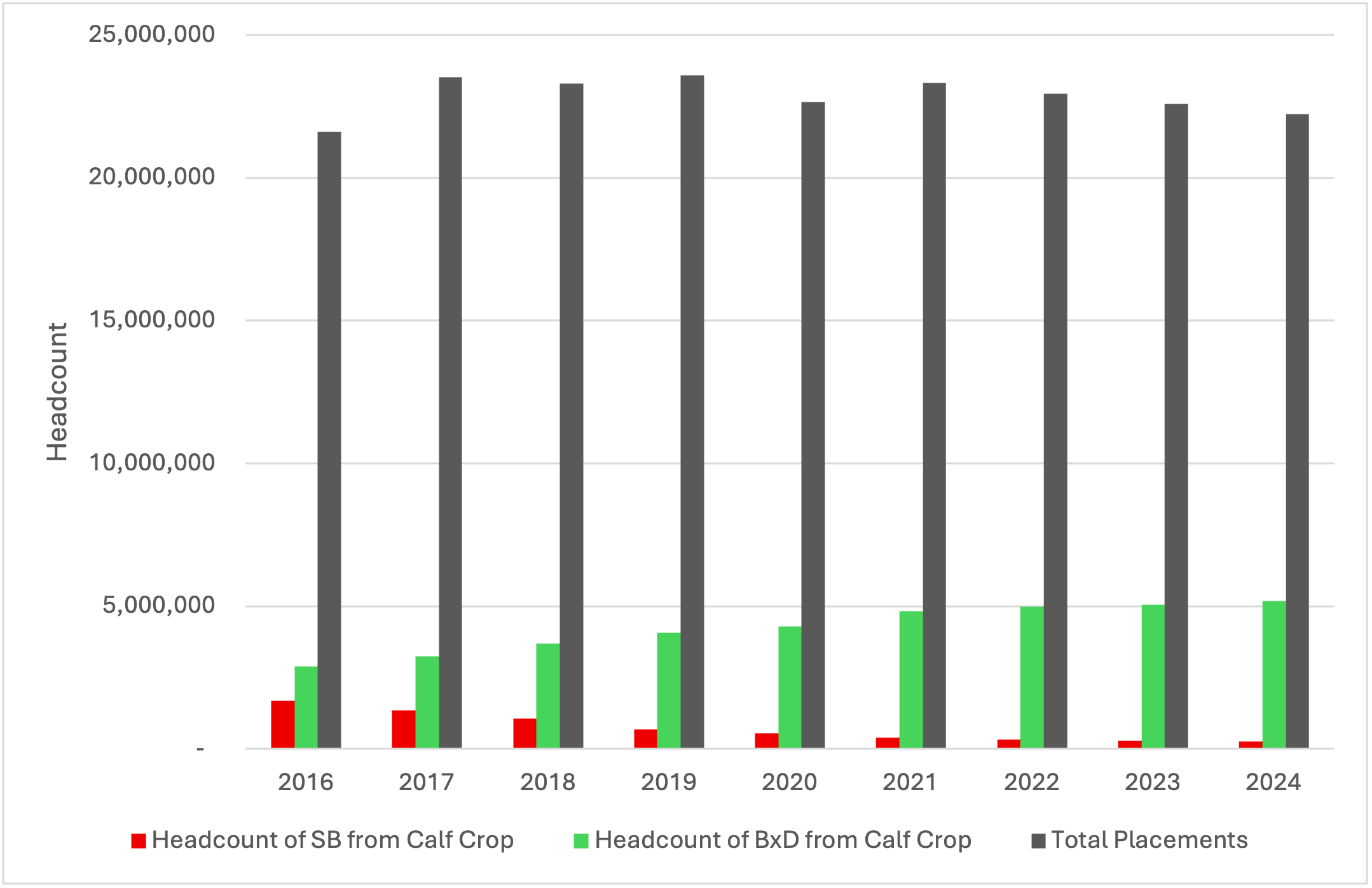
    Table 2 displays the annual percent of placements that could have been BxD cattle. Current estimates show roughly 23% of the total calf crop in 2024 was available for beef on dairy. This number has increased from 13% in 2016.

    Table 2. Annual Percent Estimates of Total Placements that are BxD Cattle

    201620172018201920202021202220232024
    13%14%16%17%19%21%22%22%23%

    Given that the national beef herd has shown no signs of rebuilding, and that the number of BxD cattle has increased each year since 2016, we can expect the percentage of placements that are BxD cattle to remain at least steady, if not to increase in the coming years. Because of this expectation, it might be beneficial for fed cattle marketing reports to indicate if marketed cattle are BxD, instead of the current reporting of them as “beef” cattle. This would also make the question posed in the introduction much easier to answer in the future. 


    Wyatt, Parker. “Beef x Dairy Placements.Southern Ag Today 5(29.2). July 15, 2025. Permalink

  • Founding Farmer

    Founding Farmer

    In light of the recent Independence Day holiday and remembering the founding fathers, there are many attributes from them that can be appreciated. 

    It is well known that many of the founding fathers had backgrounds in agriculture. Ben Franklin and James Madison were early proponents of sustainable farming. Thomas Jefferson had a penchant for plants and scientific experimentation. George Washington dabbled in all of those but was also known to be a meticulous bookkeeper. These records were considered essential in determining the success of his enterprises. 

    Due to these records and historical preservation efforts, we catch a glimpse of Washington’s efforts in farm management. They were without the digital technologies we enjoy so the records were kept entirely by hand. Day-to-day activities often got recorded in “waste books, pocketbooks, day books or memorandum books”, not unlike a typical pocket notebook farmers may utilize today. Later, the notes from these books would make it into a more formal recording known as a “journal of accounts”. If enterprises became large or complex enough, there were ledgers of accounts and even an accountant to handle these tasks. Washington, however, recorded all the transactions himself. He did so following accounting manuals such as John Mair’s Book-Keeping Methodiz’d

    While referring to his records and correspondence, Washington noted that after dinner “I resolve …[to] retire to my writing table and acknowledge the letters I have received; but when the lights are brought, I feel tired, and disinclined to engage in this work, conceiving that the next night will do as well; the next comes, and with it the same causes for postponement, & effect; and so on.” A sentiment that perhaps many a farmer can understand. However, it is evident Washington did find time for these tasks as he required large desks and bookcases to accommodate all his files. 

    Washington’s records were thorough, as evidenced by the number of documents still available and the detailed entries found on the pages. The documents are being reviewed and catalogued as part of preservation efforts through George Washington’s estate, Mount Vernon. This includes the ‘Washington as Bookkeeper’ article and The George Washington Financial Papers Project used as references for this article. That Washington continued to keep his own books and records when, almost certainly later in life, he could have had someone handle these tasks indicates the level of importance Washington placed on the contents. 

    Washington made comments throughout his decorated career on desiring to return to Mount Vernon, “I had rather be on my farm than be emperor of the world”. That Washington desired to relinquish his political power and return to humbler occupations is one reason we admire him today. To think that he would spend a considerable portion of his time recording day-to-day activities at Mount Vernon seems almost unfathomable. Let us admire his dedication, and that we can benefit from his records and example in present day.   


    Burkett, Kevin. “Founding Farmer.Southern Ag Today 5(29.1). July 14, 2025. Permalink

  • Preserving America’s Heritage Crops: Low Consumer Awareness Makes Market-Based Conservation Challenging

    Preserving America’s Heritage Crops: Low Consumer Awareness Makes Market-Based Conservation Challenging

    Heritage crops, grown from open-pollinated old cultivars, are more than just food—they embody history, culture, and biodiversity (Bessière, 2023; Britwum & Demont, 2022; Preston et al, 2012;). They can strengthen ecosystem resilience by attracting a wide range of pollinators to the agricultural field (Preston et al., 2012) and offer valuable genetic diversity that plant breeders can use to improve future crops (Wincott, 2018). 

    In the U.S., over 200 heritage foods have been cataloged by Slow Food USA (Slow Food USA, 2024). Among them, nearly 100 are originated from the Southeastern U.S. Examples include Carolina Gold rice, Sea Island red peas, and Green Glaze collards. Southeastern states such as Georgia, South Carolina, Louisiana, and Alabama have long traditions of growing heritage specialty crops, many of which thrive in the warm and humid conditions characteristic of the region. 

    Despite their cultural and ecological value, heritage crops can be more costly to grow than modern alternatives. Growers may require a price premium for this to be a profitable crop production choice. A recent national consumer survey indicates that over half of U.S. consumers are either unaware or only slightly aware of heritage varieties (Figure 1). Importantly, when we isolate responses from the Southeastern U.S., consumer awareness is similar to the national average, suggesting a critical challenge to preserve heritage crops through market‐based conservation strategies. Americans show a moderate willingness to pay a premium for heritage rice and tomato, while they are less inclined to pay more for heritage apple, cabbage, and squash (Nian et al., 2025). To safeguard these crops, integrated strategies are essential:

    • Consumer education campaigns should highlight the cultural heritage, nutritional benefits, and environmental contributions of these crops—especially in Southern states where traditional foodways remain strong.
    • Geographic indication labeling can help Southern growers develop place-based branding (e.g., “Carolina Golden Rice” or “Appalachian Beans”) that commands higher market value.
    • Public investment in regional seed conservation, grower support networks, and direct-to-consumer marketing can reduce risk and increase profitability for producers willing to diversify with heritage crops.

    In summary, heritage crops represent a unique opportunity for the Southern U.S. to lead in place-based sustainable agriculture that honors the past while preparing for the future. By bridging the gap between tradition and innovation, we can ensure that heritage crops remain a vibrant part of the U.S. agricultural future.

    Figure 1. US consumers’ knowledge of heritage crops

    Data source: Nian et al. (2025)

    References

    Bessière, J. (2013). ‘Heritagisation’, a challenge for tourism promotion and regional development: an example of food heritage. Journal of Heritage Tourism8(4), 275-291. https://doi.org/10.1080/1743873X.2013.770861.

    Britwum, K., & Demont, M. (2022). Food security and the cultural heritage missing link. Global Food Security.  35, 100660https://doi.org/10.1016/j.gfs.2022.100660.

    Nian, Y., Lamie, R.D., Vassalos, M., Tregeagle, D., Boyles, B., & Vossbrinck, D. (2025). A diamond in the rough: Identifying heritage crop niche markets in the U.S. using a discrete choice experiment. Agricultural Economicshttps://doi.org/10.1111/agec.70043

    Preston, J. M., Maxted, N., Sherman, R., Munro, N., & Ford-Lloyd, B. V. (2012). What’s in a name: a closer look at heritage variety definition. In Agrobiodiversity conservation: Securing the diversity of crop wild relatives and landraces (pp. 152-160). Wallingford UK: CABI. https://doi.org/10.1079/9781845938512.0152

    Slow Food USA. (2024). Ark of Taste | Slow Food USA. https://slowfoodusa.org/ark-of-taste/.

    Wincott, A. (2018). Treasure in the vault: The guardianship of ‘heritage’ seeds, fruit and vegetables. International Journal of Cultural Studies21(6), 627-642. https://doi.org/10.1177/1367877917733541.


    Nian, Yefan, Daniel Tregeagle, Dave Lamie, and Michael Vassalos. “Preserving America’s Heritage Crops: Low Consumer Awareness Makes Market-Based Conservation Challenging.” Southern Ag Today 5(28.5). July 11, 2025. Permalink

  • U.S. Agriculture Could Face New Challenges with President Trump’s Proposed Tariffs on Japan and South Korea

    U.S. Agriculture Could Face New Challenges with President Trump’s Proposed Tariffs on Japan and South Korea

    According to the most recent data on U.S. and China reciprocal tariffs, as reported by the Peterson Institute for International Economics (Bown, 2023), U.S. tariffs on imports from China currently stand at 51.1%, while Chinese tariffs on U.S. goods are at 32.6%. This is an improvement compared to the tariff levels in late April and early May that exceeded 100%. However, these tariffs have had a significant impact on U.S. agricultural exports to China. China is among the top five export destinations for U.S. agricultural exports (Mexico, Canada, China, Japan, and South Korea). China experienced the most significant decrease among the top markets, with exports plummeting by 55.0%, from $11.1 billion in 2024 (YTD: January – May) to just $5.0 billion in 2025 (See Table 1). This sharp drop highlights the impact of geopolitical tensions, tariff disputes, and shifting global supply chains.

    This Monday (July 7, 2025), President Trump announced on Truth Social that the U.S. will impose a 25% tariff on imports from Japan and South Korea, effective August 1st (Fortnam, 2025). This move marks a significant shift in trade policy, targeting two major allies and the 4th and 5th largest destination markets for U.S. agricultural exports. While the tariffs are intended to address bilateral trade deficits and protect U.S. industries, this decision is likely to strain diplomatic relations and could have a significant impact on U.S. agricultural exports similar to what we have experienced with China. Unlike China, U.S. agricultural exports to Japan and South Korea showed positive growth in 2025 YTD. Japan’s imports increased by 6.0%, rising from $5.5 billion to $5.8 billion in 2025. South Korea had the highest growth among the top markets, with a 15.8% increase, from $3.8 billion to $4.4 billion in 2025 (See Table 1). This surge reflects South Korea’s expanding market for U.S. agricultural goods, driven by favorable trade agreements and growing consumer demand. 

    U.S. agricultural exports to Japan and South Korea totaled $11.9 billion and $8.5 billion in 2024, respectively. Japan is a major market for U.S. corn ($2.7 billion), beef products ($1.9 billion), pork products ($1.4 billion), and soybeans ($1.0 billion). South Korea is a significant market for U.S. beef products ($2.2 billion), pork products ($0.7 billion), and corn ($0.7 billion) (USDA, 2025). If President Trump imposes a 25% tariff on imports from Japan and South Korea, U.S. agricultural trade with these countries could face significant challenges. Japan and South Korea are the 3rd and 4th largest markets for U.S. agricultural exports, showing positive growth in recent years. The tariffs could lead to reduced demand for U.S. products, harming American farmers. Additionally, Japan and South Korea might retaliate with their own tariffs on U.S. goods, further exacerbating the situation and disrupting established trade relationships.

    Table 1. U.S. Agricultural Exports, Total and Top Destinations: 2024 and 2025 (January – May)

    Country2024Jan – May 2024Jan – May 2025% Change
    $ billion
    World (total)$176.4$74.2$72.2-2.6
    Mexico30.212.512.3-1.7
    Canada29.512.011.6-3.2
    China24.411.15.0-55.0
    Japan11.95.55.86.0
    South Korea8.53.84.415.8
    Source: U.S. Department of Agriculture (2025)

    For more information:

    Bown, C.P. (2025). US-China Trade War Tariffs: An Up-to-Date Chart. Peterson Institute for International Economics. https://www.piie.com/research/piie-charts/2019/us-china-trade-war-tariffs-date-chart

    Fortnam, B. (2025). “Trump tells Japan, Korea he’s imposing 25 percent tariffs as of Aug. 1.” Inside U.S. Trade (July 7, 2025) https://insidetrade.com/daily-news/trump-tells-japan-korea-he-s-imposing-25-percent-tariffs-aug-1 (subscription required for access).

    U.S. Department of Agriculture (USDA) (2025). Global Agricultural Trade System. Foreign Agricultural Service. https://apps.fas.usda.gov/gats/default.aspx


    Muhammad, Andrew. “U.S. Agriculture Could Face New Challenges with President Trump’s Proposed Tariffs on Japan and South Korea.” Southern Ag Today 5(28.4). July 10, 2025. Permalink

  • Monthly Variability in U.S. Cotton Exports

    Monthly Variability in U.S. Cotton Exports

    Exports are an important source of demand for U.S. cotton. From 2015-2024, the U.S. has exported an average of 13.6 million bales per year, 85% of annual cotton production (USDA FAS-PS&D). The monthly variation in U.S. cotton exports is tied to production cycles and global demand.  In particular, U.S. export variation is directly tied to the U.S. production cycle, and indirectly to the production cycles of other top producing countries who are also major consumers, e.g., China, India, and Pakistan. Figure 1 shows the 10-year average (2015–2024) monthly percent of total annual U.S. cotton export value by month, along with values reported from January to April 2025. Historically, March through May are peak months for U.S. cotton exports, with March (12.5%), April (11.1%), and May (10.9%) accounting for the highest monthly average percent of total annual export value. This may indicate that the weekly export sales pace during the Spring months may be important positive determinants of March and May ICE cotton futures prices. After May, exports begin to decline, reaching their lowest point in October (4.1%). In the final months of the year, export values increase in November (5.1%) and December (7.4%).

    Figure 1. Percent of Total U.S. Cotton Export Value by Month, 10-Year Average (2015-2024) and 2025 Value by Month  

    Data Source: USDA Foreign Agricultural Service (USDA FAS) Global Agricultural Trade System (GATS)

    U.S. Cotton Exports to China, Canada, and Mexico

    U.S. cotton exports to China follow a similar pattern as the global U.S. exports. Export values peak in March (12.1%) and reach a low in October (3.8%; Figure 2). For Canada and Mexico, export sales are more consistent month-to-month (Figure 3). The stable pattern of U.S. exports to Canada and Mexico is likely due to proximity and the U.S. being the main supplier (although Mexican domestic production would be a competitor with U.S. production). U.S. cotton exports to Canada are significantly lower in quantity and value compared to exports to China and Mexico, but are relatively stable across the calendar year, with minimal variation between months. From January to April, monthly export values remain between 7.5% and 7.9%, with a peak in May. Mexico also has consistent import levels across months, with a slight peak at 9.2% in March and September and the lowest percent in December (6.2%). 

    Figure 2. Percent of U.S. Cotton Export Value by Month to China, 10-Year Average (2015-2024) and 2025 Value by Month  

    Data Source: USDA Foreign Agricultural Service (USDA FAS) Global Agricultural Trade System (GATS)

    Figure 3. Percent of U.S. Cotton Export Value by Month to Canada and Mexico, 10-Year Average (2015-2024) and 2025 Value by Month  

    Data Source: USDA Foreign Agricultural Service (USDA FAS) Global Agricultural Trade System (GATS)

    U.S. Cotton Exports to the Rest of the World (ROW; World minus China, Canada, and Mexico)

    U.S. exports to countries other than Canada, Mexico, and China grouped as the Rest of World (data not shown) follows a similar seasonal pattern as global trends displayed in figure 1. Spring marks the strongest months with March (12.9%), April (11.4%) and May (11.5%) accounting for a large portion of annual export value. However, towards the end of the year there is a significant decrease in September (4.5%), October (3.7%) and November (4.3%).

    References

    USDA Foreign Agricultural Service (USDA FAS) Global Agricultural Trade System (GATS)

    Accessed at: https://apps.fas.usda.gov/gats/ExpressQuery1.aspx

    USDA Foreign Agricultural Service (USDA FAS) Production, Supply, and Distribution (PS&D) Accessed at: https://apps.fas.usda.gov/psdonline/app/index.html#/app/advQuery