Southern Ag Today

Blog

Relating Crop and Livestock H-2A Labor Decisions to AEWR and Sectoral Wage Gaps

This article extends the regional and industry concentration analysis of H-2A patronage trends laid out in a previous Southern Ag Today article. Given the larger shares of the Southern region and crop industries in total H-2A employment figures, we offer some wage-based explanations for these patronage trends.

H-2A employment decisions are anchored on the adverse effect wage rate (AEWR) principle, which was conceived to specifically revert any possible market anomaly when foreign workers are hired under the H-2A program. The Department of Labor (DOL) was tasked to issue a fixed wage rate (AEWR) to mitigate adverse effects on local labor market conditions that may be caused by the employment of underpaid alien workers. A current year’s AEWR is determined based on the results of the previous year’s Farm Labor Survey conducted by the U.S. Department of Agriculture (USDA) among farms with annual sales of $1,000 or more (USDA, 2023). For farm work not devoted to herding or production of livestock on the range (non-range occupations that comprise the bulk of H-2A employers),^[1] AEWRs are set at the state level and enforced to apply to all workers regardless of nationality.

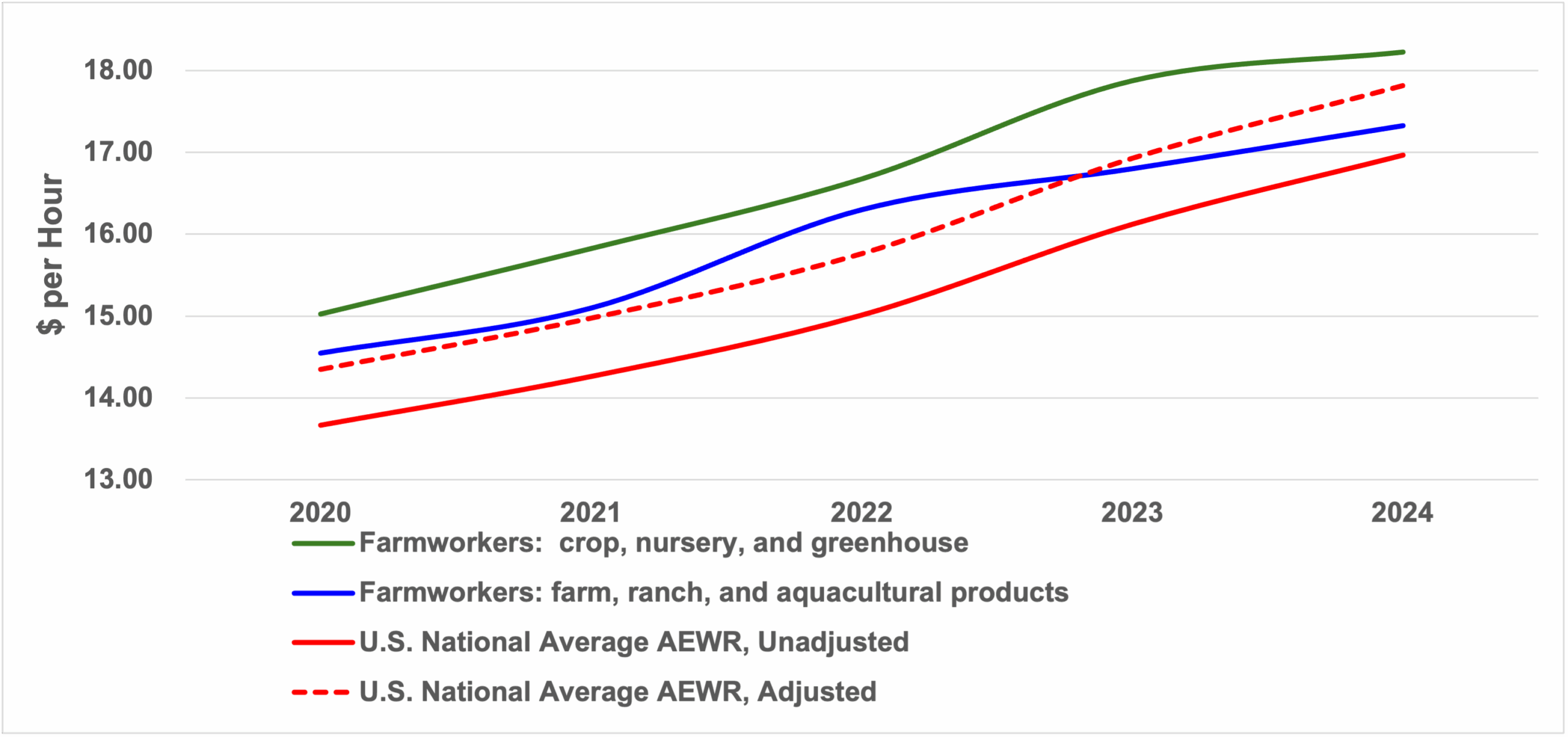
Figure 1 plots national average wages over a five-year period (2020-2024) for two farm work positions: farmworkers in crop, nursery, and greenhouse operations (usually accounting for more than 80% of all H-2A workers hired) and farmworkers in farms producing ranch and aquacultural products (which are positions held by about 4% of all H-2A workers). These wages are compared to the national average of state-level AEWRs.  An adjusted AEWR level is added to the analysis to account for discrepancies between labor remuneration packages offered to domestic and H-2A workers.  The latter not only receive wages conforming to the AEWR benchmark but are also provided with housing, transportation, meal allowances, and fringe benefits as mandated by the program.  The plots in Figure 1 indicate that crop, nursery, and greenhouse workers were consistently paid higher than H-2A workers in all years, while the adjusted H-2A wages only exceeded average livestock wages in 2023 and 2024.

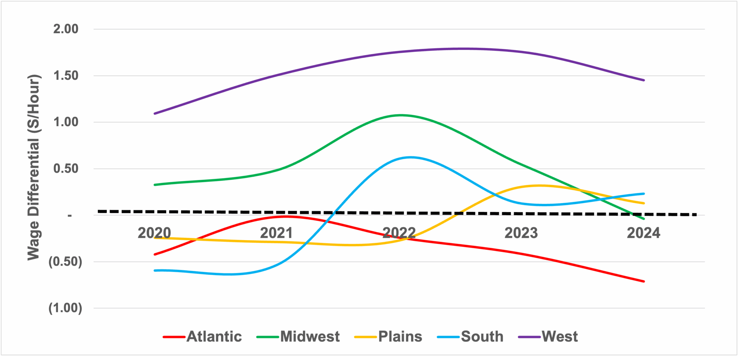
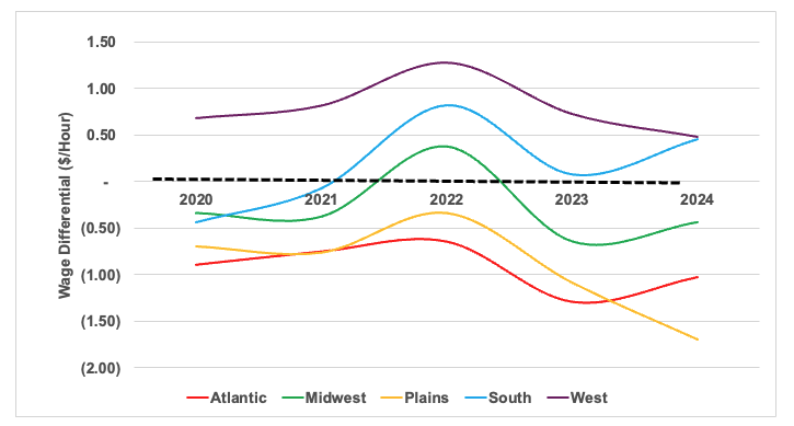
The regional wage analyses provide some deviations from the earlier trends (Figure 1), which could be influenced by regional variations in demographic, structural, and economic conditions affecting H-2A employment decisions. Figures 2 and 3 present plots of the domestic wage-AEWR differentials using regional average field and livestock wages, respectively, over the same five-year period.  In these plots, a positive gap indicates a higher regional field/livestock wage than its average AEWR.

In Figure 2 (field workers’ wages), the South region’s wage differential is positive only in 2022, while remaining negative in other years. The West, which is the second most popular regional H-2A employer, has consistently maintained a positive field wage-AEWR gap in all years. These trends indicate that while the West farms’ decisions to hire H-2A workers for field work may be motivated by wage considerations (where H-2A labor is cheaper than domestic labor), the South’s decision to hire more expensive H-2A field workers in certain years could have been driven by non-wage factors. Some analysts argue that the higher labor productivity of more expensive H-2A workers rationalizes some farms’ preference for these workers.

In Figure 3, the South posted slightly negative domestic livestock wage-AEWR differentials in 2020 and 2021; it maintained a positive gap for the rest of the period.  The West again maintained a positive gap during the entire period. These trends reveal some unique employment predicaments in livestock industries. Given that livestock farms in the country usually rely less on H-2A labor and would rather employ domestic residents, these decisions persist even when domestic livestock wages are higher than the adjusted AEWR.  Compared to crop farms, livestock farms are more inclined to seek workers and employ them for a longer tenure as their operations have longer business and production cycles.  These farms usually lure prospective workers with training offers that could upgrade their skills and job classification (from unskilled to better paying skilled positions).  A follow-up article will present more detailed evidence on livestock farms’ domestic and foreign labor hiring practices.

Figure 1.  Adverse Effect Wage Rates (AEWRs) and Farmworkers’ Wages in Crop and Livestock Farms, U.S. Average, 2020-2024

Sources:  National Agricultural Statistics Service, U.S. Department of Agriculture and Department of Labor

Note: Adjusted AEWRs include a 5% wage premium of AEWR over domestic wages as determined by Calvin, Martin, and Simnitt (2022).   These authors estimate that when all H-2A fringe benefits are factored into the equation, these foreign workers receive a wage premium of $2.55 per hour over their domestic counterparts.  However, H-2A employers are not liable to pay Social Security or Federal Unemployment Insurance taxes, thus realizing an 8% saving on payroll taxes.  Such tax benefit minimizes the H-2A-domestic wage differential to just about 5 percent.

Figure 2.  Gaps Between Adverse Effect Wage Rates (AEWRs) and Field Workers’ Wages, By Production Region, 2020-2024

Sources:  National Agricultural Statistics Service, U.S. Department of Agriculture and Department of Labor

Notes:  (1)  The regional classification of U.S. states are as follows:  ATLANTIC states include North Carolina, Virginia, West Virginia, Maryland, Connecticut, Massachusetts, New York, Vermont, New Hampshire, Maine, New Jersey, Rhode Island, and Delaware; MIDWEST states are Minnesota, Iowa, Wisconsin, Illinois, Missouri, Indiana, Ohio, Pennsylvania, and Michigan; PLAINS states are Nebraska, Kansas, Texas, North Dakota, South Dakota, and Oklahoma; WEST states include California, Washington, Oregon, Idaho, Montana, Wyoming, Colorado, New Mexico, Arizona, Utah, Nevada, Alaska, and Hawaii; and the SOUTH states are Arkansas, Florida, Georgia, Louisiana, Mississippi, Alabama, Tennessee, South Carolina, and Kentucky.

            (2) The Wage Gaps are calculated as the difference between Field Workers’ Wages and AEWR.  A positive gap indicates that field workers’ wages are higher than AEWR.

Figure 3.  Gaps Between Adverse Effect Wage Rates (AEWRs) and Livestock Workers’ Wages, By Production Region, 2020-2024

Sources:  National Agricultural Statistics Service, U.S. Department of Agriculture and Department of Labor

Notes:  (1)  The regional classification of U.S. states are as follows:  ATLANTIC states include North Carolina, Virginia, West Virginia, Maryland, Connecticut, Massachusetts, New York, Vermont, New Hampshire, Maine, New Jersey, Rhode Island, and Delaware; MIDWEST states are Minnesota, Iowa, Wisconsin, Illinois, Missouri, Indiana, Ohio, Pennsylvania, and Michigan; PLAINS states are Nebraska, Kansas, Texas, North Dakota, South Dakota, and Oklahoma; WEST states include California, Washington, Oregon, Idaho, Montana, Wyoming, Colorado, New Mexico, Arizona, Utah, Nevada, Alaska, and Hawaii; and the SOUTH states are Arkansas, Florida, Georgia, Louisiana, Mississippi, Alabama, Tennessee, South Carolina, and Kentucky.

            (2) The Wage Gaps are calculated as the difference between Livestock Workers’ Wages and AEWR.  A positive gap indicates that livestock workers’ wages are higher than AEWR.’

^[1] Distinctions in AEWR-setting are made between range and non-range occupations. Non-range workers are employed under jobs with the following Standard Occupational Classification (SOC) titles:  graders and sorters of agricultural products; agricultural equipment operators; farmworkers and laborers in crop, nursery, and greenhouse; farmworkers in the farm, ranch, and aquacultural animals; packers and packagers (hand); and all other agricultural workers (Congressional Research Service, 2023).

References:

Calvin, L., P. Martin, and S. Simnitt. (2022). Adjusting to Higher Labor Costs in Selected U.S. Fresh Fruit and Vegetable Industries. EIB-235, Economic Research Service, U.S. Department of Agriculture, Washington, DC.

Congressional Research Service. (2023) Adverse Effect Wage Rate (AEWR) Methodology for Temporary Employment of H-2A Nonimmigrants in the United States. Washington DC.  Available online at https://crsreports.congress.gov | IF12408. Accessed on August 3, 2023.

Escalante, Cesar L., and Alejandro Guitierrez-Li. “Relating Crop and Livestock H-2A Labor Decisions to AEWR and Sectoral Wage Gaps.” Southern Ag Today 5(18.1). April 28, 2025. Permalink

April 28, 2025
Members Are the Key to Cooperative Success

Arguably, farmer-owned cooperatives are the lifeblood of agriculture in the United States. They help agricultural producers to overcome a lack of market power, guarantee access to markets and services, and improve overall financial well-being from ownership of the supply chain. As long as American agriculture is composed of a relatively large number of small producers of undifferentiated commodities, cooperatives will remain a needed part of the industry. But what, in turn, is the lifeblood of your local cooperative? Members!

A cooperative is a business that is owned and controlled by the people who use it. More than just customers, these members have responsibilities to their cooperative that relate to use, ownership and control, and finance. The success or failure of a cooperative hangs on proper attention to these responsibilities.

I. Use

Cooperative members have a responsibility to use their cooperative. Cooperatives strive for greater volume of business to help them achieve profitable economies of scale. A member’s use of their cooperative sounds like the easiest of responsibilities to fulfill. However, many cooperative owners have difficulty with this. I believe the problem is that they haven’t fully adopted the owner mentality. They see their relationship with their cooperative as just another customer opportunity, meaning that when short term price opportunities arise, they quickly abandon the business that they own in favor of a competitor. This then leads many cooperative managers to exclaim, “There is no member loyalty today”.

The lesson? Members need to remember that their ownership of the cooperative represents future profitability, more stable returns, access to needed markets and services, and general protection from powerful buyers and sellers that are not invested in their future. Cooperative managers must also learn – members have no incentive to be loyal if the only benefit you offer them is based on price. Successful cooperatives also pursue excellence in customer service and product quality and will continually educate members on the value of cooperation.

II. Ownership and Control

Cooperative members have a responsibility to exert the rights of ownership and control over their cooperative. Each member of the cooperative is an owner and should understand their cooperative in all aspects – its structure, bylaws, policies, operations, legal obligations, and financial status. Occasionally, I am approached by an individual with a great idea for a business and who thinks a cooperative business structure would be best. Most of those cases fail to progress when we discuss member-ownership and control.

Cooperatives are formed by members based on their needs. Members incorporate the business – not management. Members elect directors, define the mission of the cooperative and establish bylaws and policies. Although members hire a general manager to operate the business and manage employees, they are still involved in controlling the business by providing direction, serving on committees, expressing opinions, and voting on significant changes to the cooperative.

The most successful cooperatives educate members about operations and the ways that the cooperative engages in business. Boards of directors often take a tour of their cooperative’s operations and come away surprised at their increased knowledge that inspires better board decisions.

III. Finance

Cooperative members have a responsibility to finance the cooperative for the purpose of conducting operations. They are not responsible for financial returns. Profitability remains the responsibility of management. Members are responsible for ensuring the business has the necessary capital to form and operate the business. This is done initially through the purchase of a share of voting stock (which gives the rights of membership). One-time investments may also be used when forming the business or expanding into new services or product lines. Ultimately, the most important means for members to finance their cooperative takes us back to use, or patronage. The greater the patronage, the greater the cost efficiency of the cooperative. It should be noted that members are responsible in sharing losses just as they are in sharing earnings.

Members make the cooperative successful. Through use, ownership and control, and finance, members are the lifeblood of their local cooperative.

Park, John. “Members Are the Key to Cooperative Success.” Southern Ag Today 5(17.5). April 25, 2025. Permalink

April 25, 2025
Does it Have to Be All or Nothing in Farm Policy?

Long before the 2018 Farm Bill expired on September 30, 2023, there appeared to be one voice among the entire U.S. food and fiber system asking Congress to get a new farm bill completed that would provide producers an improved safety net with meaningful protection from low prices, bad yields or both.  Since that time, the economic condition of U.S. crop farms has deteriorated significantly due to low prices and high costs as reported in Southern Ag Today here and here.  Now, the farm bill appears to be stalled behind other priorities, namely a budget reconciliation bill that will provide the funding needed to extend the expiring Trump tax cuts that were enacted in the President’s first term and to beef up border security, among other priorities.

As part of the budget reconciliation process, the instructions to the House Agriculture Committee were to cut $230 billion from the baseline over ten years while the instructions to the Senate Agriculture Committee were to cut at least $1 billion over ten years.  Figure 1 provides estimates of the 10-year baseline from FY 2025 to FY 2034 to provide some perspective on projected spending across farm bill titles.  The expectation is that Title IV (the nutrition title) of the farm bill is where the majority of savings will originate.  It should be noted that the farm bill that passed out of the House Agriculture Committee last year and the Senate Republican farm bill proposal added around $55 billion (House) and $40 billion (Senate) in spending above the baseline to make the safety net stronger, in addition to other enhancements.

It appears that some parts of the House and Senate farm bill proposals might be able to be added to the budget reconciliation bill.  The exact details of how that might happen are not entirely clear, but it does appear that option is being considered.  Suffice it to say that, in our opinion, that is the only realistic pathway to achieving meaningful enhancements to the farm safety net for the 2025 crop.  There are some who worry this might fragment the farm/food coalition that has generally worked together to get a farm bill across the finish line.  We would, however, point out that the coalition fell apart during the 2014 Farm Bill debate in the House of Representatives, where two separate bills (a nutrition bill and a farm-only bill) had to be passed out of the full House and then combined again during the conference process with the Senate.  While we recognize the importance of all parts of the farm bill, in the name of trying to protect a very vulnerable crop production sector, Congress may wish to consider moving away from all or nothing this time around.

Figure 1.  Farm Bill Titles with Mandatory Baseline, 10-Year Projected Outlays, FY2025-FY2034, billions.

Source: Congressional Research Service, What Is the Farm Bill?, RS22131, Updated April 9, 2024.  Available at https://www.congress.gov/crs_external_products/RS/PDF/RS22131/RS22131.81.pdf

Outlaw, Joe, and Bart L. Fischer. “Does it Have to Be All or Nothing in Farm Policy?” Southern Ag Today 5(17.4). April 24, 2025. Permalink

April 24, 2025
Incrementally Pricing Corn into a Futures Market Rally

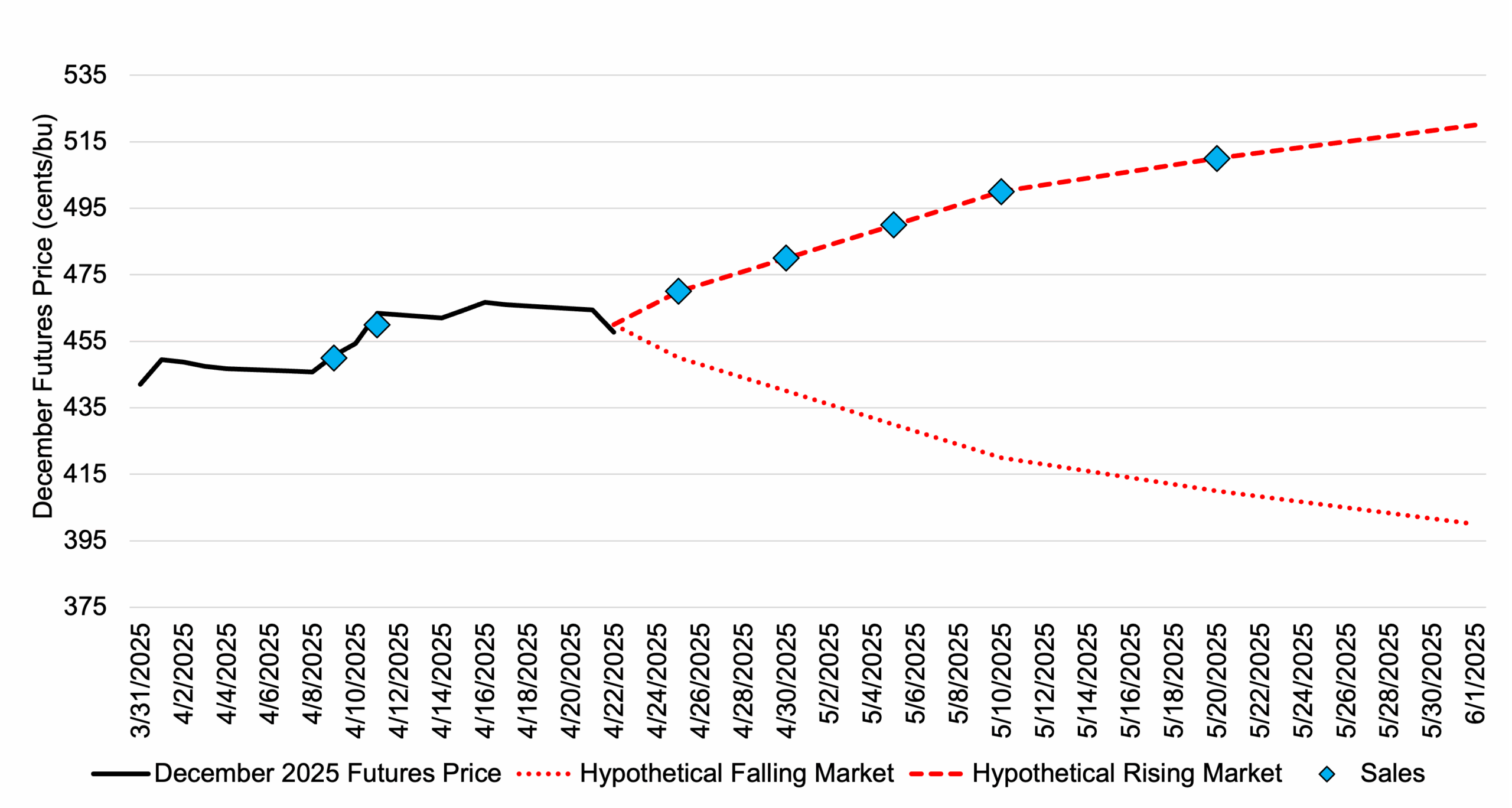
Tariff escalation remains a major source of uncertainty that could substantially move corn futures markets in the coming weeks/months. Managing some futures price risk based on the current rally is worth considering given the uncertainty in corn markets. On Friday April 11, December corn futures broke through a key resistance point at $4.60/bu. For those farmers that have not started pricing the 2025 crop, December corn futures above $4.50/bu represent a good starting point to remove some futures price risk (basis could be secured now or left to be fixed at an alternative date depending on local basis offerings). Pricing into a futures market rally, through incremental sales, is a strategy worth considering, and one that will take some of the emotion out of marketing decisions. For example, starting at a December futures price of $4.50/bu, consider pricing 5% of projected 2025 production. For each additional 10-cent increase in futures price, consider establishing a futures price on an additional 5% of estimated production up to a maximum of 35% of projected 2025 production. Pricing more than 35% of the crop before June can be risky and can result in exchanging price risk for production risk or having limited production to price should a bullish weather market occur in June/July/August. The maximum amount to be priced before June can be a personal preference based on the farmers’ risk tolerance, variability in yield for the farm, and access to storage. This incremental pricing strategy would establish an average futures price of $4.80/bu on 35% of projected production if the December corn futures price rallied to $5.10/bu (Figure 1). However, it would also put some sales (10% of estimated production at an average price of $4.55/bu as of April 22) on the books if the current rally stalled or reversed. Futures prices above $4.50 plus a positive basis, which occurs in most Southern states, will result in cash prices of nearly $5.00.

Table 1. December Corn Futures Price and Sales into a Hypothetical Rising or Falling Market

References and Resources:

Barchart.com. December Corn Futures Price. Accesses April 22, 2025. https://www.barchart.com/futures/quotes/ZCZ25/interactive-chart.

Smith, Aaron. “Incrementally Pricing Corn into a Futures Market Rally.” Southern Ag Today 5(17.3). April 23, 2025. Permalink

April 23, 2025
Fewer Heifers in Feedlots

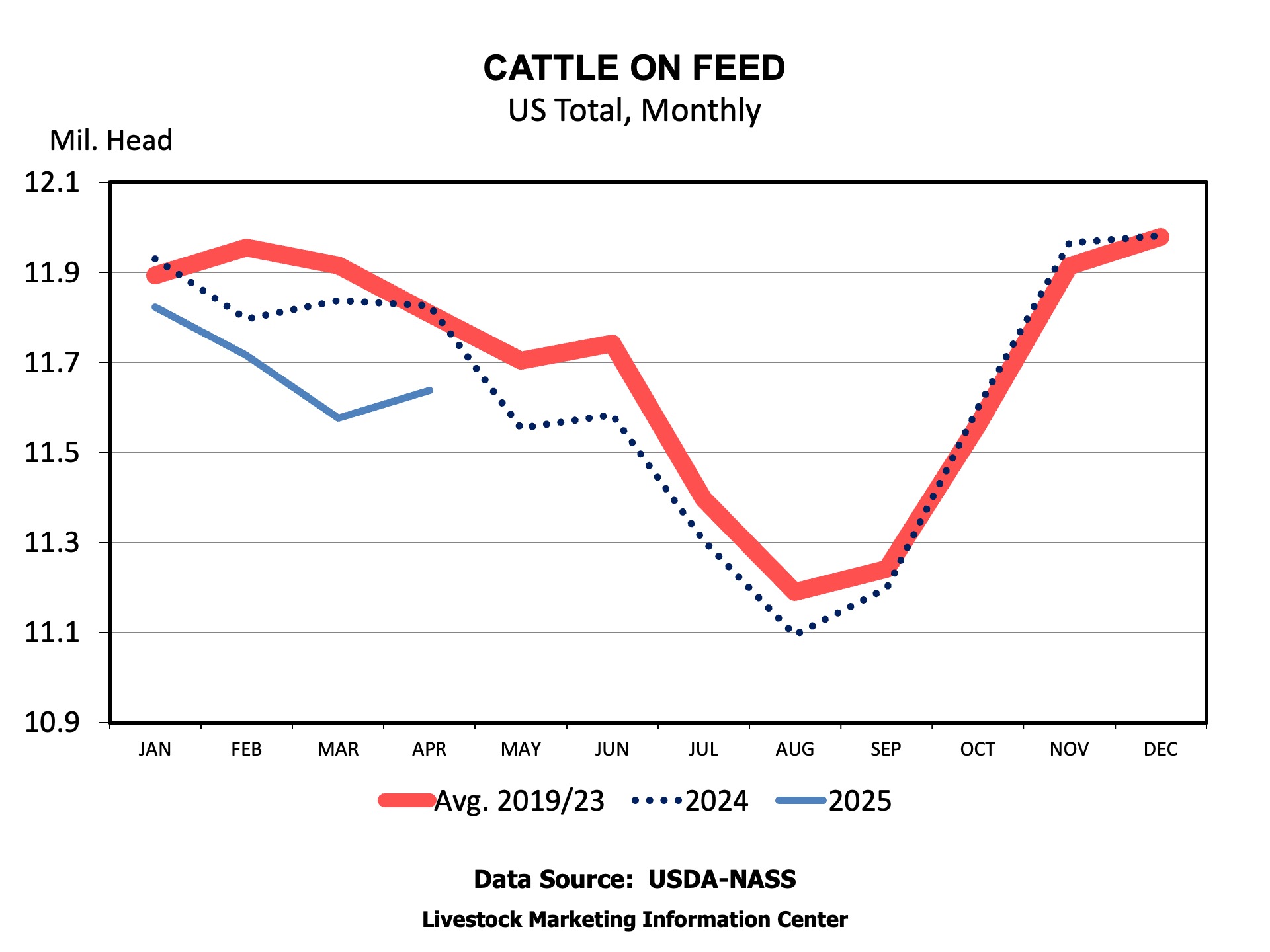
The headline numbers of feedlot marketings, placements, and total cattle on feed were not a lot different from expectations.  Feedlot marketings in March were just over 1 percent larger than the previous March.  With the same number of working days in the month as last year, daily average marketings slightly outpaced a year ago.  Placements were 5.1 percent larger than last year.  Larger placements were not a surprise due to an expectation that placements were delayed a bit from February and, normal, seasonally larger March placements from wheat and other small grain pastures.  Larger placements and marketings left the total number of cattle on feed 1.6 percent fewer than last year.

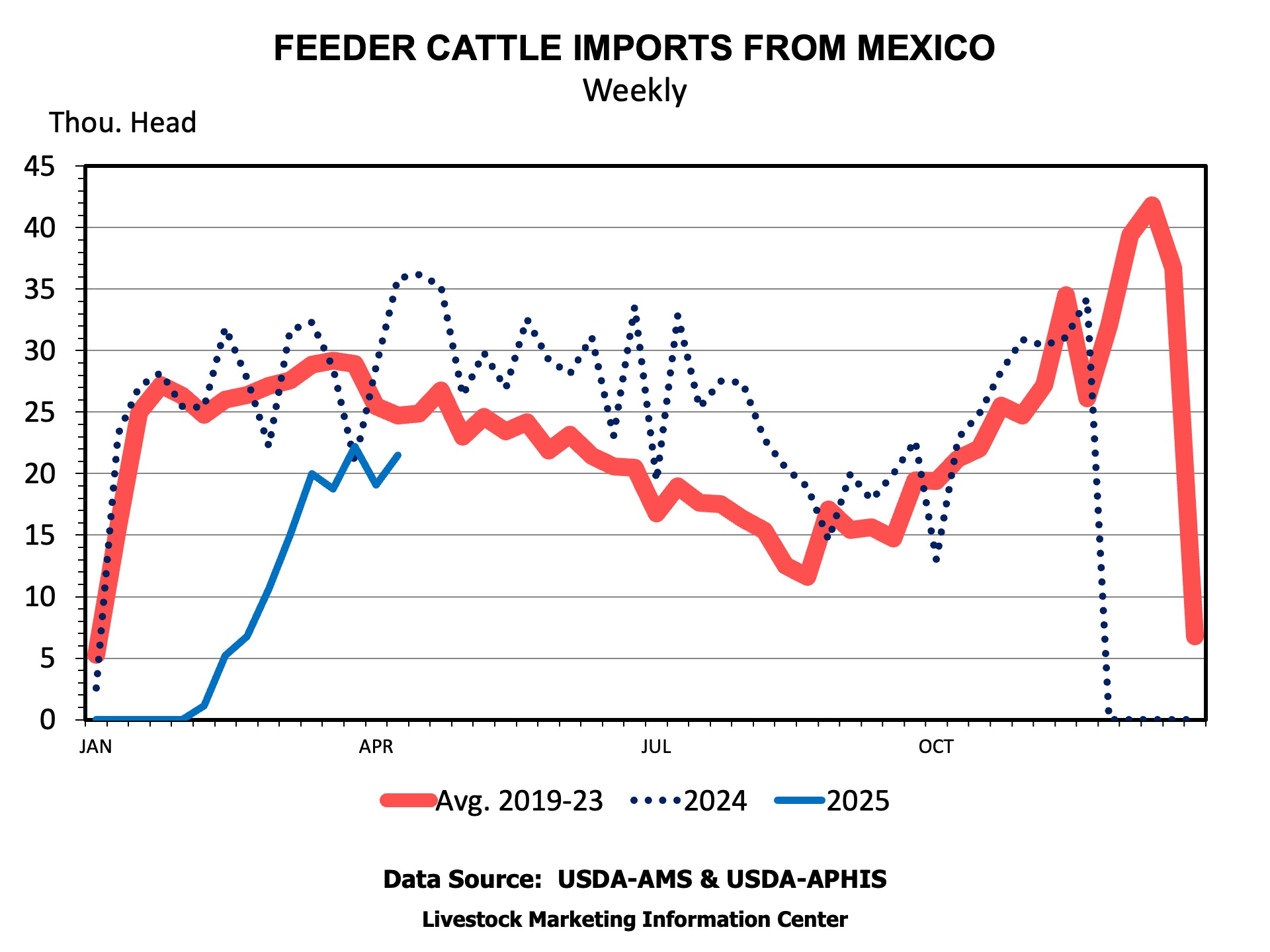
Placements for the year are worth another look.  For the first 3 months of the year, placements are 4 percent, or 216,000 head, fewer than last year.  But, feeder cattle imports from Mexico through March are down 227,000 head compared to a year ago.  Remember that there were no imports through January and much slower imports in February due to screwworm regulations.  Taken together, the decline in imports from Mexico is larger than the total decline in placements so far this year.  The impact of fewer feeders from Mexico likely shows up in Texas’ placements, which are down 13.1 percent for the year.

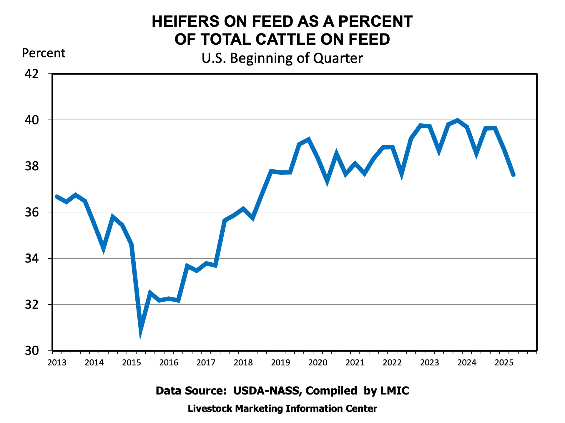
To save the best for last, the most interesting part of this report was the quarterly estimate of the number of heifers in feedlots on April 1.  Heifers on feed were down 4 percent, or 180,000 head, compared to April 2024. The 4.38 million heifers on feed were the fewest since April 2020 and before that, April 2018.  Since the first of the year, 77,000 fewer spayed heifers were imported from Mexico, so they make up a portion of that decline.  While the headline of fewer heifers on feed may raise eyebrows, the number remains large.  There have been more than 4 million heifers on feed for 30 consecutive quarters, and they make up 37.6 percent of the cattle on feed.  We’ll have to wait for larger and consecutive declines in heifers on feed as evidence of any heifer retention for herd rebuilding.

Anderson, David, and Josh Maples. “Fewer Heifers in Feedlots.” Southern Ag Today 5(17.2). April 22, 2025. Permalink

April 22, 2025