While the vast majority of beef produced in the U.S. is consumed domestically, international markets are a significant piece of the U.S. beef system. For perspective, the U.S. exported the equivalent of about 12.5% of its beef production during 2022, while importing roughly 12%. This was a fairly typical balance of trade, especially for a year with high beef production levels like last year. However, as beef production is on track to see a significant drop in 2023, trade patterns are also being impacted.
Through August, exports of U.S. beef are down by 14% from the first eight months of 2022. A drop of that magnitude certainly warrants some question but is largely a case of year-over-year comparison being a little misleading. For the first two quarters of 2023, beef production was about 4% lower than 2022. With lower production levels, a larger share of U.S. production will be consumed domestically. Additionally, high price levels are also making imports of U.S. beef less attractive in many countries. For example, exports to our three largest destinations (South Korea, Japan, and China) are all down sharply so far this year.
The same factors that have led to lower export levels have also led to an increase in U.S. beef imports. Through the first eight months of the year, U.S. beef imports are up by a little over 5%. The largest percentage increases are in beef imports from Australia, New Zealand, and Uruguay, which are primarily sources of lean trim to go into ground beef. Unlike 2022 when the U.S. was a slight net exporter of beef, we are very much on track to be a significant net importer in 2023. Through August, U.S. beef imports have exceeded exports by more than 20%.
This trend towards increased imports and decreased exports is likely to continue for the next few years. Given that this calf crop is smaller than last year’s calf crop, beef production is likely to decrease in 2024. And given expectations for lower beef cow inventory next year, I would expect beef production to be lower again in 2025. The same supply fundamentals supporting strong cattle prices are resulting in a significant shift in the balance of trade for beef. And as beef supplies get increasingly tighter over the next couple of years, we are likely to see an ever greater divergence between imports and exports.
World wheat production exceeded world wheat consumption for 7 out of 8 marketing years from the 2013/14 marketing year to 2019/20. The stocks-to-use ratio as measured by days of use on hand at the end of the marketing year increased from a 104-day supply to 146 days on hand over the same period. Since 2020/21, we have seen four consecutive years of total use greater than production. Days on hand have subsequently fallen back to a 119-day supply. During this period, Russia invaded Ukraine in February 2022, raising concerns over exportable wheat supplies from the critical Black Sea wheat producing region.
As world wheat supplies tightened, cash wheat prices doubled from the summer of 2020 to the fall of 2021, from just under $4 per bushel to $8, then to over $12 in the months after the invasion. Prices have since fallen back to levels last seen in the summer of 2021 (the early stages of the 2021/22 marketing year). This price retracement has occurred even though world days of use on hand at the end of the marketing year are lower, and the conflict in Ukraine continues.
Figure 1. Texas Cash Wheat Prices, weekly
A key factor behind prices moving lower despite tightening world wheat fundamentals is the continued movement of wheat from the Black Sea region. In the marketing year prior to the invasion, Russia and Ukraine exported 56 mmt of wheat, 28% of world wheat exports. Current estimates for the 2023/24 marketing year are for combined exports of 60 mmt, 29% of the world total.
This export total is a result of record wheat exports from Russia and a 50% reduction in exports from Ukraine. Russia has gone from virtually no wheat exports in the 2000/2001 marketing year to a projected 49 mmt in the 2023/2024 marketing year. (Figure 2) Export capability comes from a 50% increase in production over the last 10 years. Further, Russia has increased production by 10 million harvested acres since 2013, and increased yields from 33 to 47 bushels per acre.
Figure 2. Russia Wheat Production, Exports, Consumption, and Ending Stocks
Russian wheat supplies are of increased importance to the world wheat market. Russia’s wheat exports have increased against a backdrop of tightening world wheat fundamentals. Wheat prices have fallen as wheat exports continue from the Black Sea region, even though the supply and demand situation for world wheat is tighter than before the Russian invasion of Ukraine. In the current world wheat supply and demand environment, any substantial limitation or reduction in exportable wheat supplies from Russia (e.g., due to reduced wheat production, export policy, or geopolitical forces) would likely result in a significantly amplified price response.
Cooperative firms return profits to their member-owners in proportion to their use of the firm. Those profit distributions are referred to as “patronage refunds”. In contrast, most other corporations distribute profits in proportion to investment. Cooperative members may be somewhat familiar with patronage refunds but often do not understand all of the structures and issues. Producers who are not a member of a cooperative may wonder what they are missing. Patronage refunds are the most unique and, perhaps, the most interesting feature of cooperatives.
In cooperative terminology, a patron is a cooperative customer who qualifies to receive patronage refunds. That typically means that they are a member of the cooperative. Patronage refunds are profits that are distributed in proportion to use. Usage can be measured in multiple ways. Patronage can be based on the dollar amount of purchases or commodity payments or on physical units such as bushels or tons. A cooperative can track member use as a single patronage pool, or as multiple pools reflecting separate commodities, products or departments. Each cooperative selects the patronage base that most fairly represents member use.
Cooperatives can pay patronage as a combination of cash and equity. Equity patronage is eventually redeemed into cash and, for that reason, is often called “revolving equity”. Equity patronage has two functions. First, it allows members to build ownership without an out-of-pocket investment. Second, it capitalizes the cooperative, funding the property, plant and equipment.
Patronage refunds have tax implications. Cooperatives are taxed as corporations but are allowed to deduct patronage distributions. Those patronage refunds become taxable income for the patrons. Cash patronage is immediately taxable to the patron but equity patronage can be structured to be taxable when issued or taxed at the later date when it is redeemed into cash.
Many local cooperatives are in turn members of regional cooperatives. Those regional cooperatives issue patronage refunds to the local cooperatives, which becomes part of the local cooperative’s net income. Therefore, the patronage refunds that producers receive from their local cooperative reflects both the local cooperative’s profits and the pass through share of the regional cooperative’s profits.
Many younger producers wonder why a cooperative cannot simply offer more favorable prices (more than what competition might dictate) in lieu of paying patronage refunds. There are some very good reasons. Equity patronage capitalizes the cooperative. One way to think of equity patronage is that the members are receiving their share of the total profits and then temporarily reinvesting a portion of those profits in the cooperative. The second rationale for not substituting favorable prices for patronage is the danger of misestimating costs and creating a loss. Finally, favorable prices would result in zero profits and zero return on assets and equity. Basically, profits have been given away in the form of prices. Many members will not perceive the price benefit and conclude that the cooperative is poorly managed. By setting prices at market level, generating profits and then returning those profits as patronage refunds, members can observe the cooperative’s performance and appreciate its benefit, and the cooperative will be capitalized and able to respond to member needs.
Most producers wish they could purchase their inputs a little cheaper and sell their commodities at a slightly higher price. Most producers would also like to invest for the future. Producers can achieve all of the goals with no out-of-pocket investment by joining and patronizing their local cooperative. When you are a cooperative patron, the check really is in the mail!
With cotton added back to the farm safety net via the Bipartisan Budget Act of 2018, the 2018 Farm Bill largely maintained the statutory reference prices (SRPs) established in the 2014 Farm Bill. One noticeable exception was the addition of Effective Reference Prices (ERPs) in the 2018 Farm Bill at the insistence of House Republican negotiators. As we noted in a December 2022 Southern Ag Today article, Section 1101 of the 2018 Farm Bill (P.L. 115-334) allows for the ERP for a commodity to replace the SRP if 85% of the previous five-year Olympic average of the national marketing year average price is greater than the SRP. The ERP may increase to as much as 115% of the SRP.
A recent article noted that the Congressional Budget Office (CBO) is projecting that “9 of the 19 program crops will have an ERP higher than the SRP in at least some of the years of the baseline” with those crops representing “over 90% of all base acres in the United States.” They argue that this will result in an increase in Reference Prices “without Congress needing to do anything more than extend those [ERP] provisions.” While the article expressed surprise at “how little attention the ERP has received,” we have been reporting on it since the inception of Southern Ag Today as noted above. It seems the real purpose of this new article was to call into question the need for higher SRPs in the next farm bill, a key request of many state and national commodity organizations across the country. We believe this latest article seriously misses the mark in two key respects:
First, while there is no question that the ERP provision is projected to result in higher Reference Prices for certain crops, it is projected to have zero impact on several other major commodities, including cotton, rice, and peanuts. While the author acknowledged this point, he simply used the absence of an increase in market prices for these other crops as a nonsensical justification for not adjusting the SRPs for these crops. As we’ve noted elsewhere (including in recent Southern Ag Today articles), sticky production costs and the prospect of lower prices are the primary justifications for increased SRPs (frankly, for all covered commodities).
Second, while ERPs are certainly projected to provide higher levels of protection for some crops, those levels will also drop if marketing year average prices fall going forward. As a result, while CBO’s relatively flat price projections are an important factor in the debate, the much more important consideration for policymakers is how the farm safety net will fare if those projections are wrong. To that end, we analyzed the impact of an unforeseen price drop on all 64 crop farms maintained by the Agricultural & Food Policy Center (AFPC) at Texas A&M University. Specifically, we examined the impact of a price decrease over the next 5 years assuming that crop prices followed the same path experienced during the last downturn from 2013 to 2017. Under this scenario, 33 of the 64 crop farms maintained by AFPC would face a greater than 50% likelihood of an ending cash shortfall at the end of the baseline outlook (2028). In other words, under that scenario, 52% of the farms would have a greater than 50% chance of exhausting all cash on hand over the next 5 years and would have to debt-finance the day-to-day operations of the farm. Bottom line: if there are any unforeseen hiccups in the market, the current farm safety net is simply NOT up to the task of mitigating losses for many farms across the country.
As we’ve noted time and again, the farm bill debate is fertile ground for those who like to sow regional discord. Serious observers know that the farm bill must work for growers throughout the United States and not just one region of the country. If the goal is to ensure that the farm safety net can provide meaningful levels of support for producers in the event of a downturn in the farm economy, simply relying on existing Effective Reference Prices – or even modest 5-10% increases in the Statutory Reference Prices for many covered commodities – will simply prove insufficient. Producers are operating in a higher cost environment, the Federal farm safety net needs to reflect that fact. We are all for the swift completion of the farm bill, but given the extraordinary amount of capital that American producers are putting at risk, we continue to believe that the substance of the farm bill is far more important than the timeline.
Although it is early in the harvest season for many crops grown in the South, it is time to begin revising your annual enterprise budgets in preparation for the 2024 growing season. Enterprise budgets are forward-looking estimates of production costs on a per acre basis for a particular enterprise and production method (e.g, cotton on non-irrigated land).
When it comes to enterprise budgets, direct operating costs are straightforward. If a grower plans to use an input, they specify the amount they plan to use per acre and multiply that by the price per unit of that input. The product is an estimate of the operating cost per acre to charge to that enterprise.
Some overhead costs, also known as ownership costs, are more complex because they are noncash expenses. One may wonder why it is important to charge noncash expenses to an enterprise. There are two reasons for this. First, the use of owned equipment causes wear and tear over time. Eventually, owned equipment needs to be replaced. The loss in value overtime, or depreciation, should be charged to the enterprise for the use of that equipment. Second, the capital invested in the equipment could be invested elsewhere and earn a percentage return on that investment. This opportunity cost, or interest expense, should also be charged to the enterprise.
One effective method of calculating these noncash overhead costs is using the capital recovery method. The capital recovery method enables growers to estimate an annual per acre cost in present day dollars based on the useful life of the equipment used by the enterprise. The following equation can be used to calculate annual capital recovery cost per acre.
-where n represents the useful life of the equipment and i represents the interest rate. The table below lists capital recovery factors (CRF) by year (n) and interest rate (i).
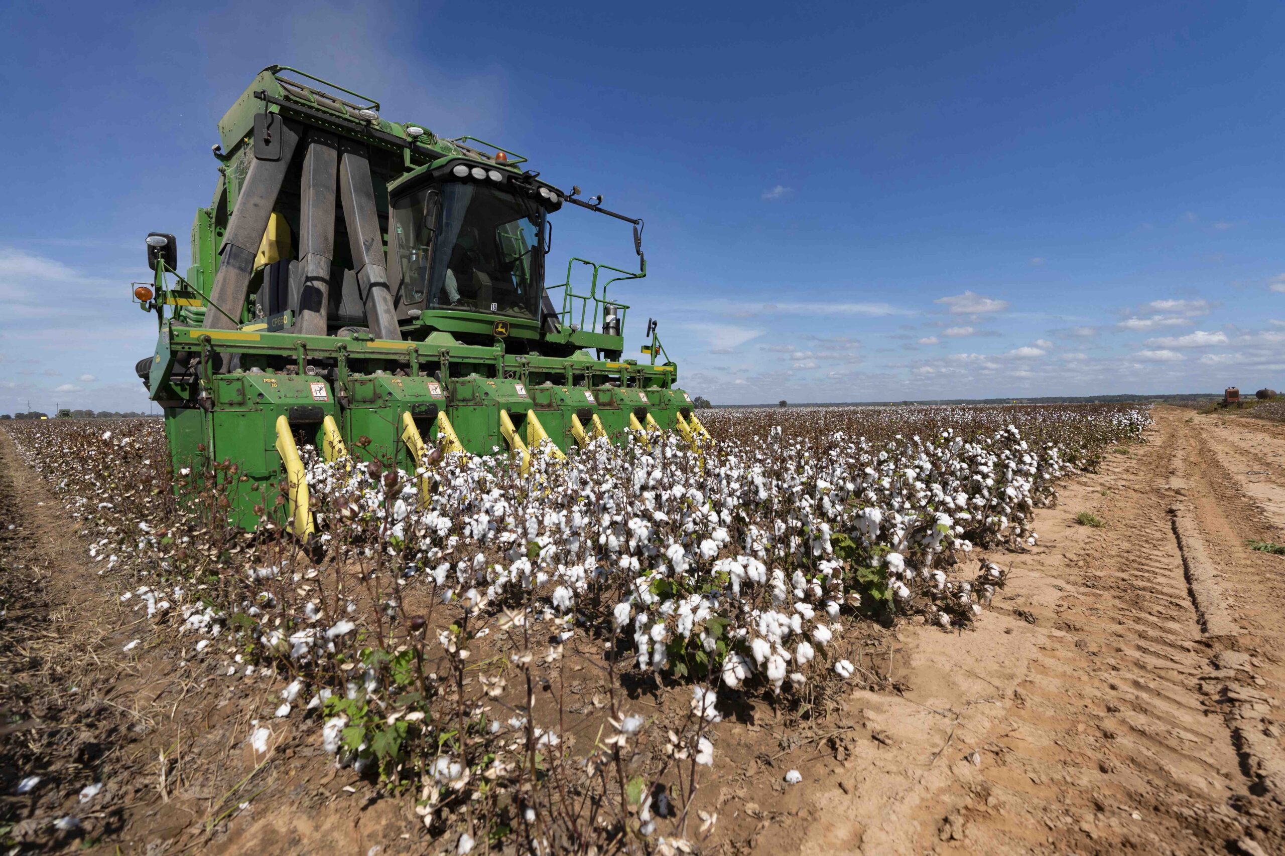
Some row crops are more capital-intensive than others because they require commodity-specific harvest equipment. This is certainly the case for cotton and peanuts in the South. Grain growers need one combine to harvest their grain, and different headers can be switched out to harvest corn, soybeans, and wheat/other small grains. Cotton farmers need a cotton picker or stripper to harvest cotton, and it cannot be used to harvest any other crop. Peanut farmers need a digger/inverter to dig and invert peanut vines and then use a peanut picker to pick the peanuts off the vines. Like cotton, peanut harvest equipment cannot be used to harvest any other crop.
Figure 1 provides an example of annual capital recovery cost per acre at different interest rates for cotton, peanut, and grain harvesting equipment. The appropriate interest rate to select depends upon the grower, their risk tolerance, and desired rate of return on their investments. The average range is between 8-10%, with 9% highlighted on the chart.
The harvest equipment used in this example are based on typical equipment sizes used in Georgia (6-row equipment on 36-inch row spacing) and are assumed to be new. Capital recovery costs can also be calculated on used equipment based on the equation above. Table 1 lists the assumptions on purchase price, salvage value, useful life, and total annual harvest acres. Note, since the harvest equipment is only being evaluated in this article, the tractor has similar total acres to the sum of the peanut digging and picking quipment which are pulled by the tractor, with some allowance for turnaround at the end of the rows. The grains combine is assumed to harvest multiple crops like corn and soybeans.
Table 1 Title: Assumptions on purchase price, salvage value, useful life, and total annual harvest acres.
Figure 1 Title: Sensitivity Analysis of the Annual Capital Recovery Cost per Acre for Cotton, Peanut, and Grains Harvest Equipment.
Chart Source: Author created, using a capital recovery factor table, data on purchase prices, and assumptions on salvage value, useful life, and annual use.
It is evident that cotton and peanuts are more capital-intensive because of the specific harvest equipment and those enterprise budgets need to account for those higher costs per acre. Furthermore, interest rates matter. As interest rates increase, capital recovery costs do too.
While this is only an example for harvesting equipment, this method should be used for each machine used in producing a specific enterprise and added together to determine the total annual capital recovery cost. Table 2 lists a range of capital recovery factors by year and interest rate to aid growers in tabulating these costs on all of their equipment owned by the farm.
Table 2 Title: Capital Recovery Factors (CRF) by Year (n) and Interest Rate (i)